2.10. Nuclei Studio Advanced Features
At https://doc.nucleisys.com/nuclei_studio_supply we maintain an extensive and continuously growing collection of usage questions and case studies for Nuclei Studio and Nuclei Tools to help you use them more effectively. Feel free to take a look.
2.10.1. Importing Projects Created by Older Versions
2.10.1.1. Importing Old Projects Into Nuclei Studio 2023.10
In Nuclei Studio 2023.10, the toolchain, SDK, and other components have changed significantly. To use a project created with an older version of Nuclei Studio, or an older SDK, in the new Nuclei Studio, follow the instructions in this section.
When you import a project created with an older version of Nuclei Studio into Nuclei Studio 2023.10 (for the detailed import procedure, see Importing Old Projects in Nuclei Studio 2022.12 and Later), or use a project created with an older SDK (that is, any SDK released before the Nuclei Studio 2023.10 release), the project is configured to use GCC 10. If the corresponding toolchain cannot be found, build errors and other problems occur, and the project does not work normally.

There are two solutions: manually import the GCC 10 toolchain, or convert the project with the conversion tool shipped with Nuclei Studio 2023.10. The second solution is recommended because it converts the project more thoroughly to a format supported by Nuclei Studio 2023.10 and lets you use its latest features.
2.10.1.1.1. Manually Importing the GCC 10 Toolchain
For convenience, Nuclei Studio 2023.10 retains the GCC 10 configuration, but GCC 10 is not packaged with the IDE. To continue developing with GCC 10, import GCC manually.
Locate GCC 10 in the toolchain\gcc\ directory of the old Nuclei Studio installation and copy its contents into the toolchain\gcc10\ directory under the Nuclei Studio 2023.10 installation directory, then rebuild the project. The project should now build normally. However, Nuclei QEMU does not work with this method; if your project requires Nuclei QEMU, manually modify the corresponding QEMU debug configuration.

2.10.1.1.2. Converting a Project to Support GCC 13 with the Tool
Nuclei Studio 2023.10 provides a quick conversion tool, Convert GCC 10 Project to GCC 13, that makes it easier to import old projects. Right-click the project and select Convert GCC 10 Project to GCC 13 from the context menu.
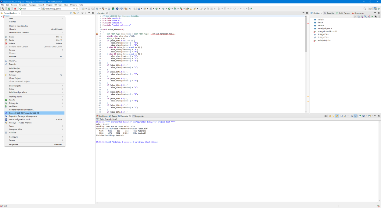
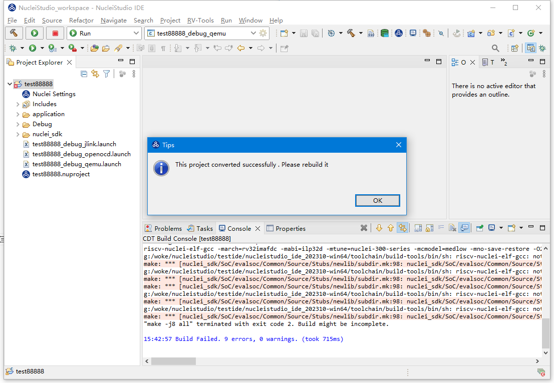
After the project is converted, rebuild it. Nuclei Studio then builds the project with GCC 13, and features such as QEMU work normally.
2.10.1.1.3. Batch Converting Projects to Support GCC 13
You can also batch convert projects to support GCC 13 in Nuclei Studio 2023.10 and later versions.
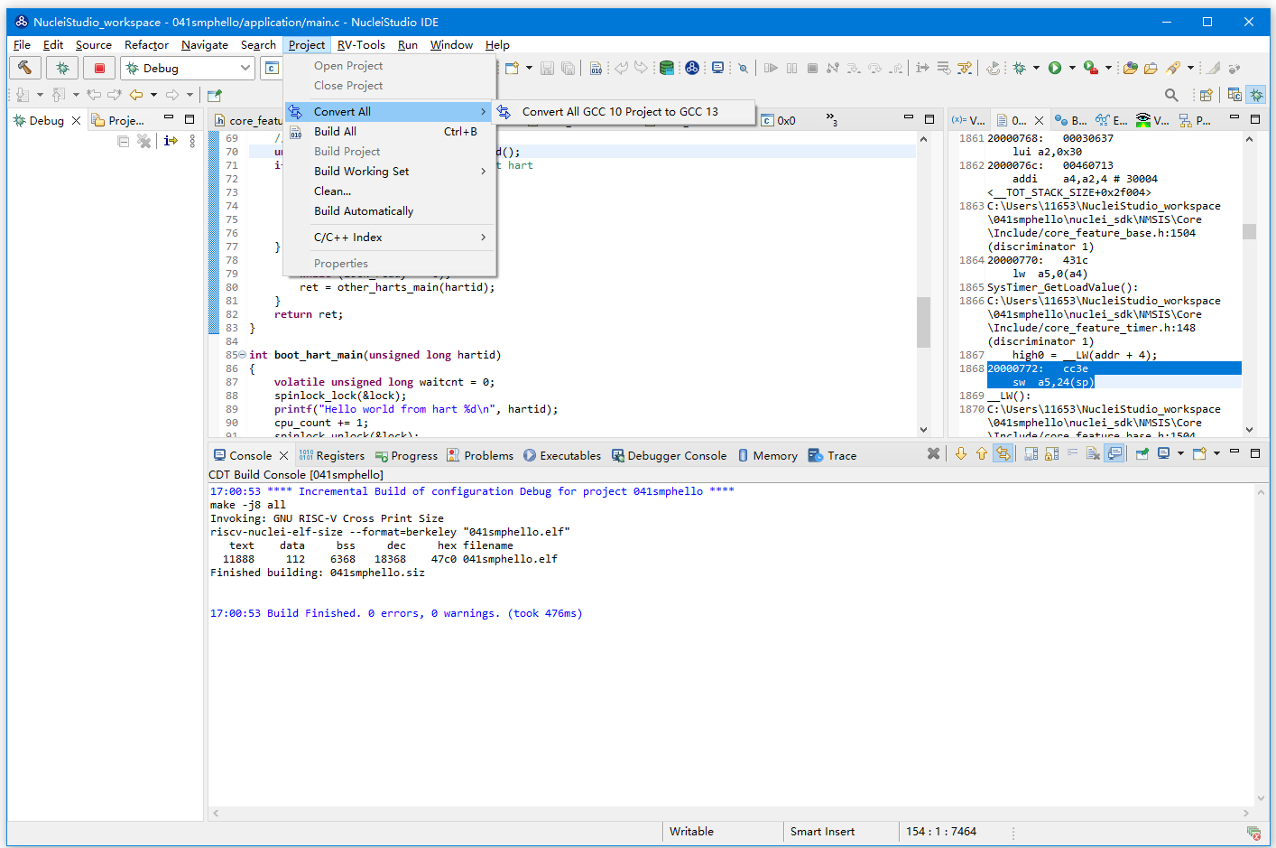
Open the conversion tool, select the projects you want to convert, and start the conversion.
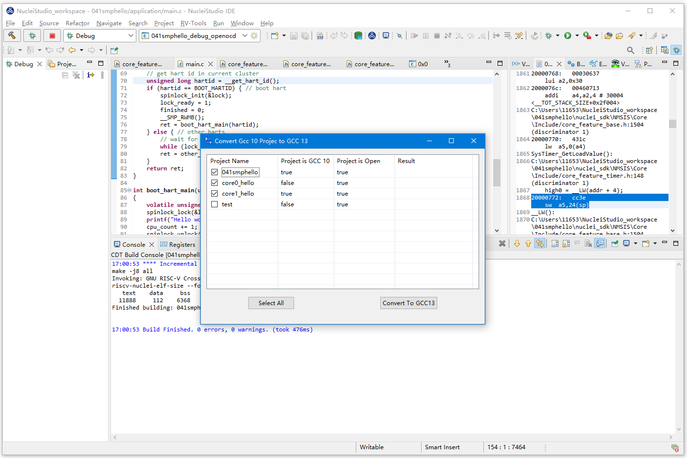
When the conversion is complete, the page displays the conversion results for each project.

2.10.1.2. Importing Old Projects in Nuclei Studio 2022.12 and Later
Nuclei Studio 2022.12 optimized project import to make project sharing easier. After a project is exported from the IDE, double-click the .nuproject file to quickly import and open it in Nuclei Studio.
First, export the project in Nuclei Studio 2022.12: right-click the project and select Export.

In the Export dialog, select General->File System and follow the wizard to export the project to the specified folder.
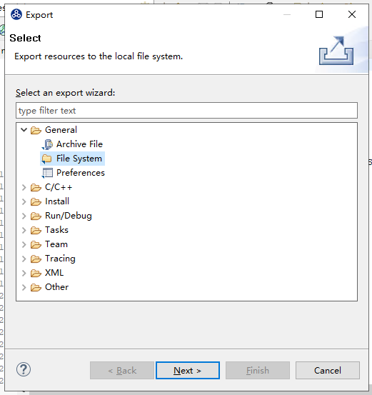
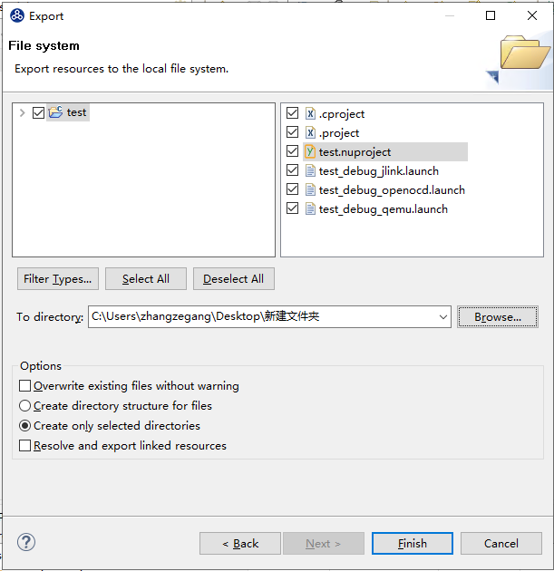
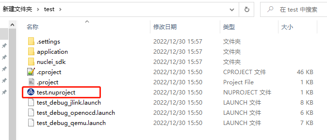
Next, import the project. The exported project contains a test.nuproject file; click this file to import the project into Nuclei Studio. For details, see Import a Project via an Application Association File.
2.10.1.3. Importing Old Projects in Versions Earlier Than Nuclei Studio 2022.12
In Nuclei Studio 2023.10, the toolchain name was changed from riscv-nuclei-elf-gcc to riscv64-unknown-elf-gcc, and the GCC version was upgraded from GCC 10 to GCC 13.
Starting with version 2020.08, Nuclei Studio upgraded its official toolchain from RISC-V Nuclei GCC (riscv-nuclei-elf-gcc) to GNU MCU RISC-V GCC (riscv-none-embed-gcc). Because the compiler prefix changed, projects created with IDE version 201909 or earlier must have their settings adjusted before they can be used in the new IDE. The following example uses a helloworld project generated with Nuclei Studio 201909 to describe the import procedure and the required settings changes:
Import the helloworld project generated with version 201909. For the detailed import procedure, see Section 5.2.
After importing the project, right-click it and select
Propertiesto open the settings page. SelectC/C++ Build -> Settings, open the Toolchains tab, and change the Name drop-down option toRISC-V Nuclei GCC (riscv-nuclei-elf-gcc). Click Apply to save the change.

Right-click the project again and select
Clean Project, thenBuild Project.
2.10.2. LST View
Nuclei Studio 2024.06 integrates the LST View tool. LST View can be used on its own or invoked from the Trace tool or the GProf tool. It helps you view LST files and link them with the source code.
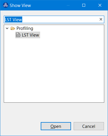
In Nuclei Studio, go to Window -> Show View -> Other and search for LST View in the Show View dialog.
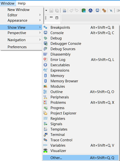
Open the LST View tool.
LST View has a toolbar at the top with a search drop-down box for entering an Addr to search for, an Open File menu that opens a file selector for choosing the .lst file to open, and a Find menu for searching within LST View.
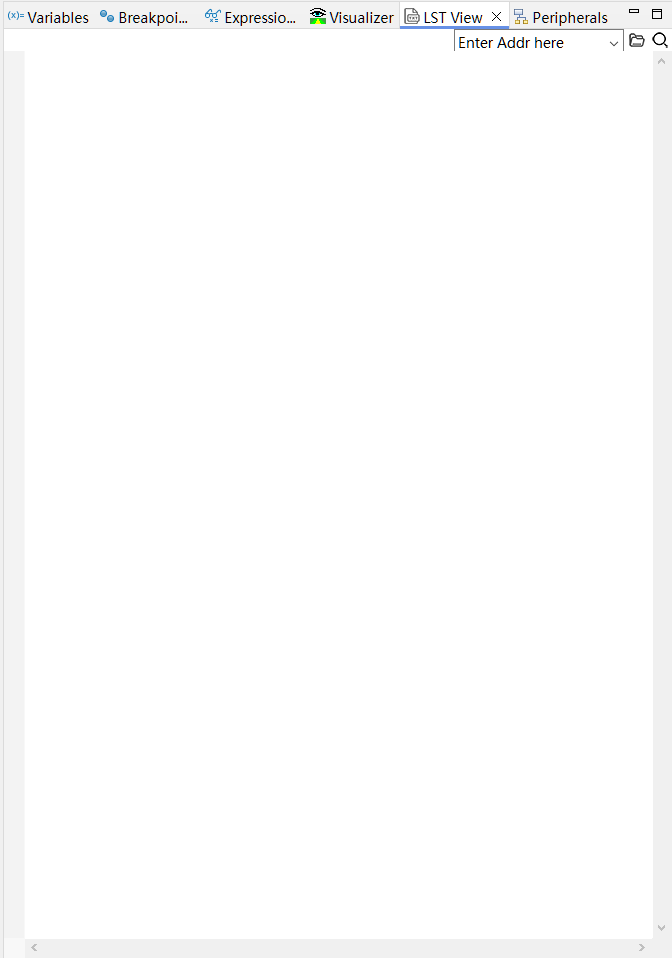
Use the Open File menu to locate the lst file in the file selector. The file is usually located in the Debug directory after the project is built.

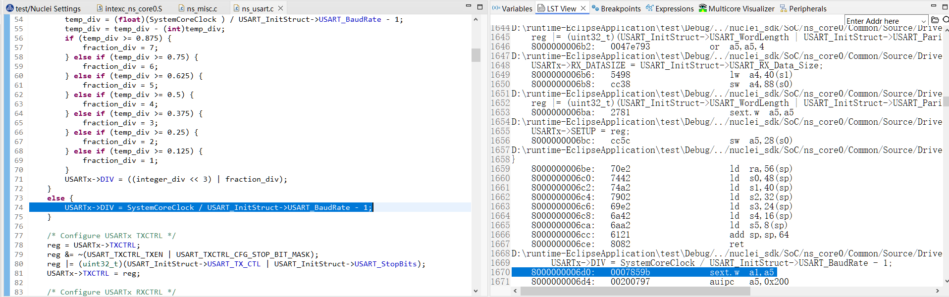
After opening the file, you can search within it. When you select a line of text that contains a valid Addr, LST View uses that Addr to locate the corresponding source file and line number, opens the source file in the editor, and places the cursor on the corresponding line. This links the source file to the lst file so you can view the two together.
2.10.3. Code Coverage and Profiling
Nuclei Studio 2023.10 and later integrates Eclipse Linux Tools, whose features have been partially optimized so that Nuclei Studio projects can use the Code Coverage and Profiling related features. In Nuclei Studio 2024.06, these features were further optimized and upgraded to make them easier to use.
For tutorials on using Coverage, Profiling, and Call Graph, see Using Coverage, Profiling, and Call Graph.
For details about Eclipse Linux Tools, see Eclipse Linux Tools
If you encounter any problems during use, check https://github.com/Nuclei-Software/nuclei-studio or submit an issue.
Note
The Nuclei System Technology WeChat Channel contains a video on How to Use Code Coverage and Profiling in Nuclei Studio. Search for the Nuclei System Technology WeChat Channel in WeChat to view it.
2.10.3.1. About Code Coverage
The Code Coverage feature in Nuclei Studio relies on the gcov tool provided by the GCC compiler to view the code coverage of specified source files. It helps developers determine whether their test cases are sufficient and cover all branches and paths of the code under test.
In Nuclei Studio, build the file or folder you want to analyze with the --coverage or -coverage compile option. When the program runs on a real development board, the semihost feature reads and writes files on the host computer, so the required coverage files (gcda/gcno files) can be collected. Alternatively, use the profiling library provided by Nuclei SDK to print the coverage data to the serial port; the IDE then parses the data and saves it to the host.
Caution
The compile option
--coverageor-coverageshould only be added to a specific application directory or source file, not to the entire project. Otherwise, the program consumes a large amount of memory at runtime and fails to run.When the 2025.02-gcc 14.x or later compilers are used together with the Nuclei SDK Profiling library (<=0.8.0), the coverage feature does not work properly and no coverage information is produced. For the fix, see https://github.com/Nuclei-Software/nuclei-sdk/commit/5aaae0d5a7629013a235657ed3bce3dce18e8e0b
Note
As of the Nuclei Studio 2025.10 release, the library implementation of Nuclei SDK 0.9.0 Profiling/Coverage does not yet support the clang compiler. If you use the clang compiler for testing, an error is reported. This should work normally once Nuclei SDK adds the related support in a future release.
Note
Due to the GCC version upgrade, projects created with the latest SDK may behave abnormally when the Code Coverage feature is enabled. This issue has been fixed in Nuclei Studio 2025.10.
Note: This fix only supports SDK version 0.8.1 and above and is not backward compatible with older projects. For projects created with an older SDK, manually modify the configuration to adapt to the new version. Refer to the changes in the following GitHub commit and adjust your project accordingly: https://github.com/Nuclei-Software/nuclei-sdk/commit/5aaae0d5a7629013a235657ed3bce3dce18e8e0b
The
.gcnofile is generated when source code is compiled with the-ftest-coverageoption of the GCC compiler. It contains information for reconstructing the basic block graph and assigning source line numbers to blocks.The
.gcdafile is generated when an object file compiled with the-fprofile-arcsoption of the GCC compiler runs. A separate.gcdafile is generated for each object file compiled with this option. It contains arc transition counts, value profile counts, and some summary information.
In general, the --coverage or -coverage option alone instructs the compiler to produce the files described above. Note that *.gcda files are produced at runtime, so the runtime environment must support file reading and writing. Here we use semihosting: the files are written to the host through the semihost feature of OpenOCD.
Note
When collecting coverage, compile with O0 so that the coverage information is as accurate as possible.
For details about the Code Coverage feature, see
2.10.3.2. About Profiling
The Profiling feature in Nuclei Studio relies on the gprof tool in the GCC compiler and binutils to view the running time and call counts of functions in a specified file, as well as their call relationships. gprof helps identify program bottlenecks for performance optimization. It collects data while the program runs and generates a report showing the percentage of CPU time each function occupies and the call relationships between functions.
In Nuclei Studio, build the specified source files with the -pg compile option. When the program runs on a real development board, the semihost feature reads and writes files on the host computer, so the required coverage files (gcda/gcno files) can be collected. Alternatively, use the profiling library provided by Nuclei SDK to print the coverage data to the serial port; the IDE then parses the data and saves it to the host.
Note
The compile option -pg should only be added to a specific application directory or source file, not to the entire project. Otherwise, the program consumes a large amount of memory at runtime and fails to run.
Producing the gmon.out file requires compiler support, and the program must actually run on a board whose runtime environment supports file reading and writing before Profiling can produce useful results.
For details about the Profiling feature, see
2.10.3.3. About Call Graph
Call Graph is a powerful tool that gives developers an intuitive view of the call relationships between functions or methods in a program. With Call Graph, developers can quickly identify frequently called functions, key entry points, and dependencies between functions. In Nuclei Studio, Call Graph obtains the program’s call relationships mainly by analyzing Profiling data.
In Nuclei Studio, go to Window -> Show View -> Other, search for Call Graph in the Show View dialog, and open the Call Graph tool. The Call Graph tool provides multiple views; the most commonly used are described below.
2.10.3.3.1. Radial View
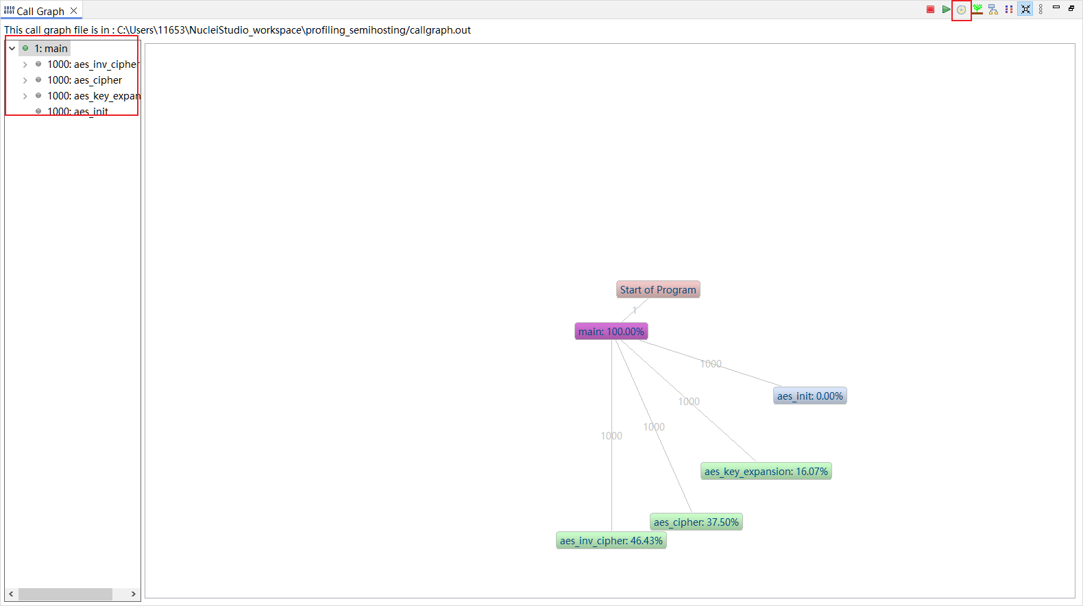
This view shows the call relationships of the program. Double-click a parent node in the menu on the left, and the area on the right displays all call relationships starting from that parent node. You can also use the menu to view the selected call relationship in the other views.
2.10.3.3.2. Tree View
Shows the call relationships, time consumption percentages, call counts, and other information for the program selected in Radial View. Select a function to view its parent nodes, child nodes, and other information.
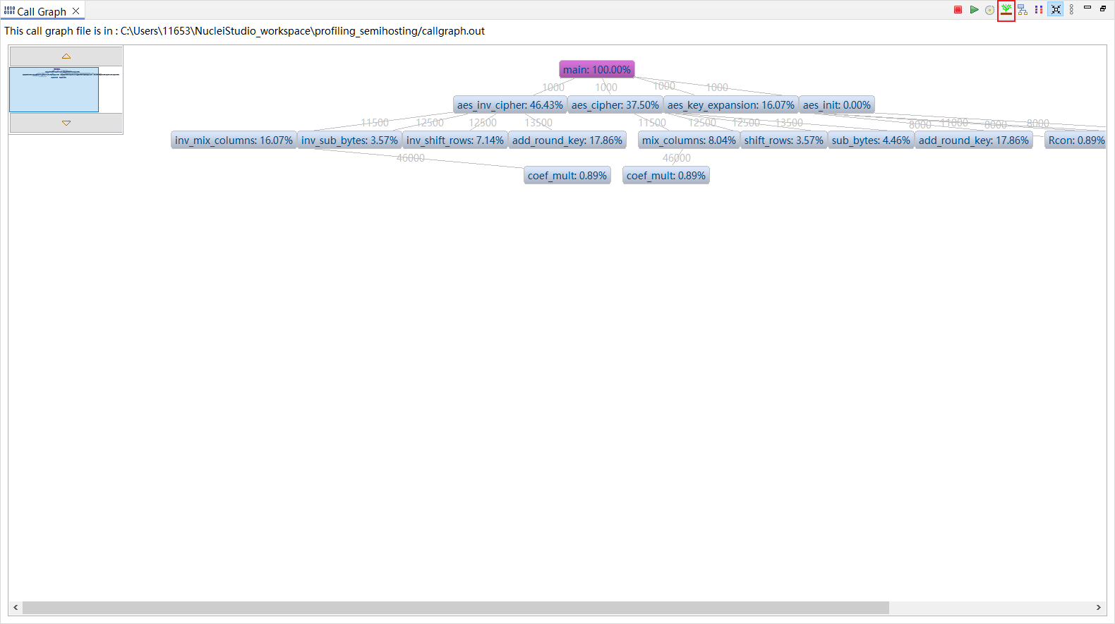
2.10.3.3.3. Level View
Similar to Tree View, it shows the call relationships and call counts of the program.
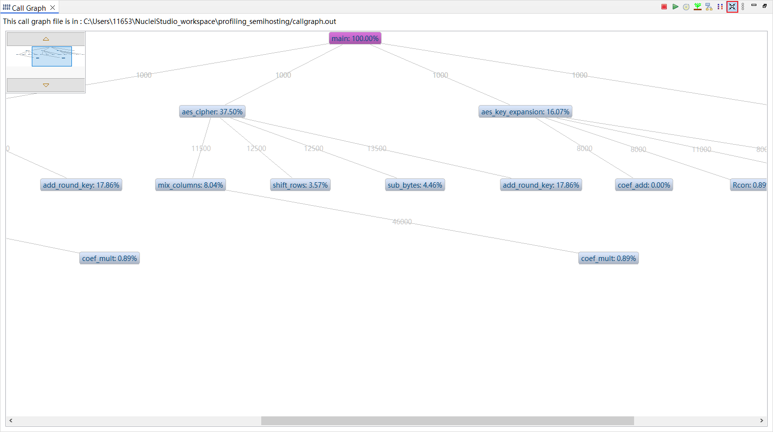
2.10.3.3.4. Aggregate View
Shows the program’s time consumption visually as a square diagram.
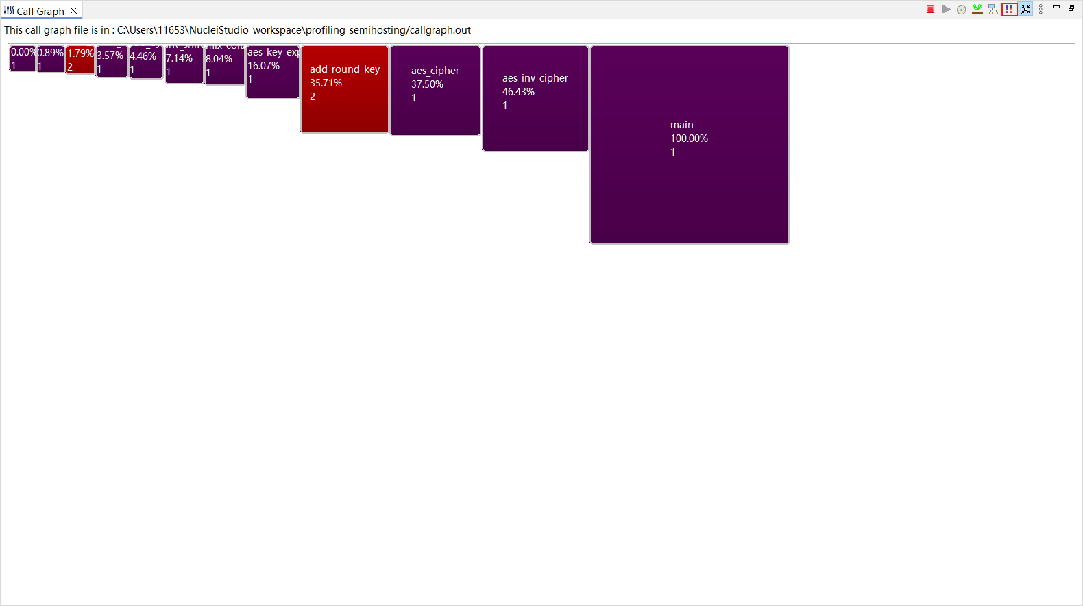
2.10.3.4. Using Coverage, Profiling, and Call Graph
Using Coverage, Profiling, and Call Graph in Nuclei Studio 2024.06 is straightforward. The following examples use Nuclei Studio 2024.06 and nuclei_sdk 0.6.0 to demonstrate two ways of using the Coverage, Profiling, and Call Graph tools.
2.10.3.4.1. Using via Serial Port
nuclei_sdk 0.6.0 and later versions include a Profiling demo to show how to use gprof and gcov test project. After installing nuclei_sdk 0.6.0 in Nuclei Studio, you can create this test project. For details about the Profiling demo to show how to use gprof and gcov test project, see demo_profiling.
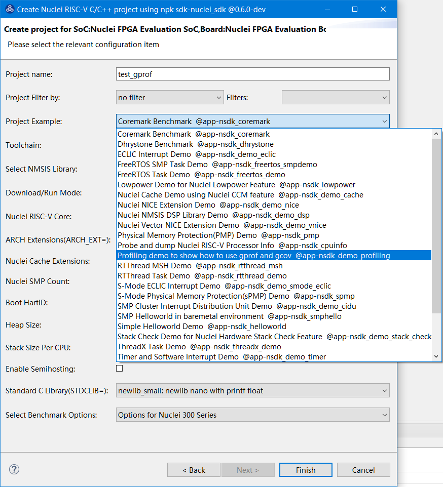
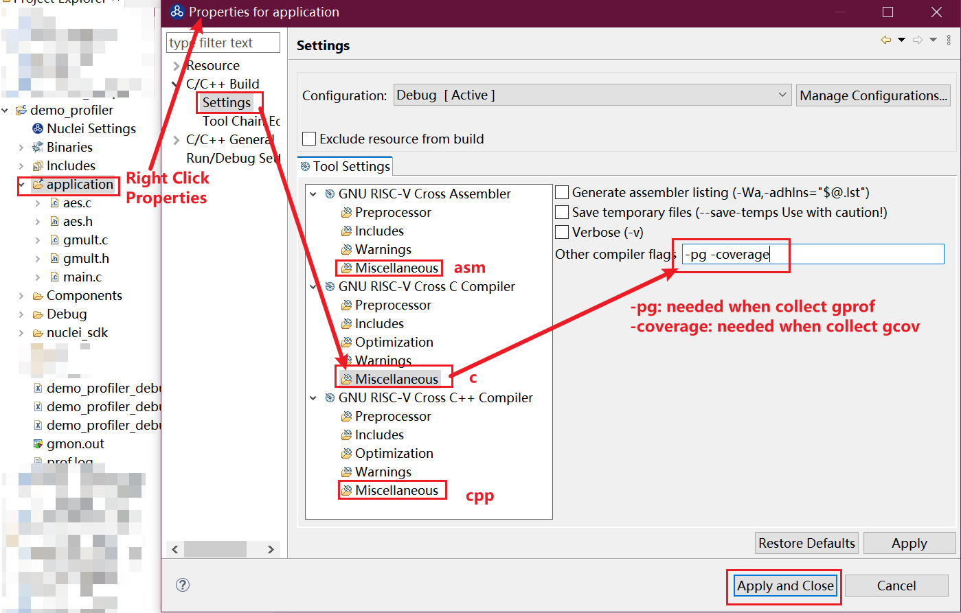
After the project is created, set the -pg, --coverage, or -coverage compile option for the files or folders you want to analyze, then build the project.
Note
The compile options -pg, --coverage, or -coverage should only be added to a specific application directory or source file, not to the entire project. Otherwise, the program consumes a large amount of memory at runtime and fails to run.
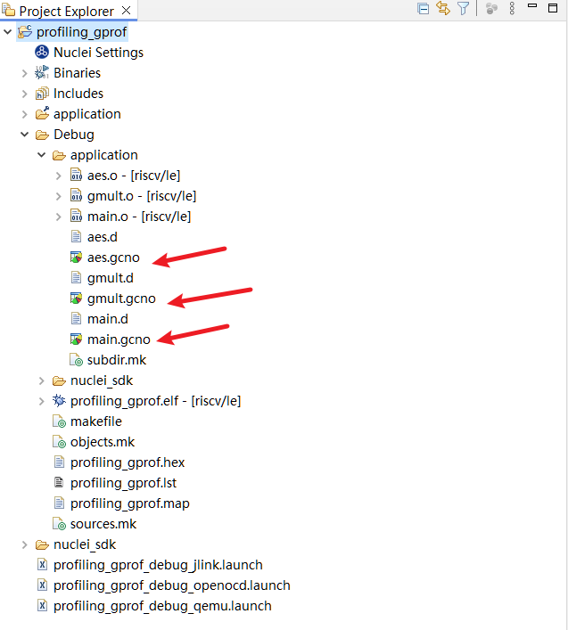
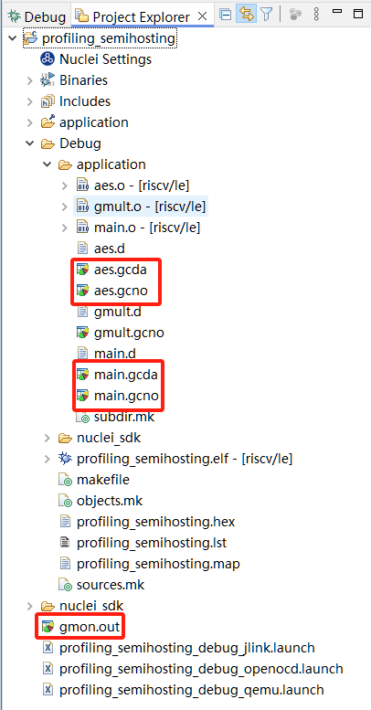
In the Debug directory of the successfully built project, you can see that several .gcno files have been generated.
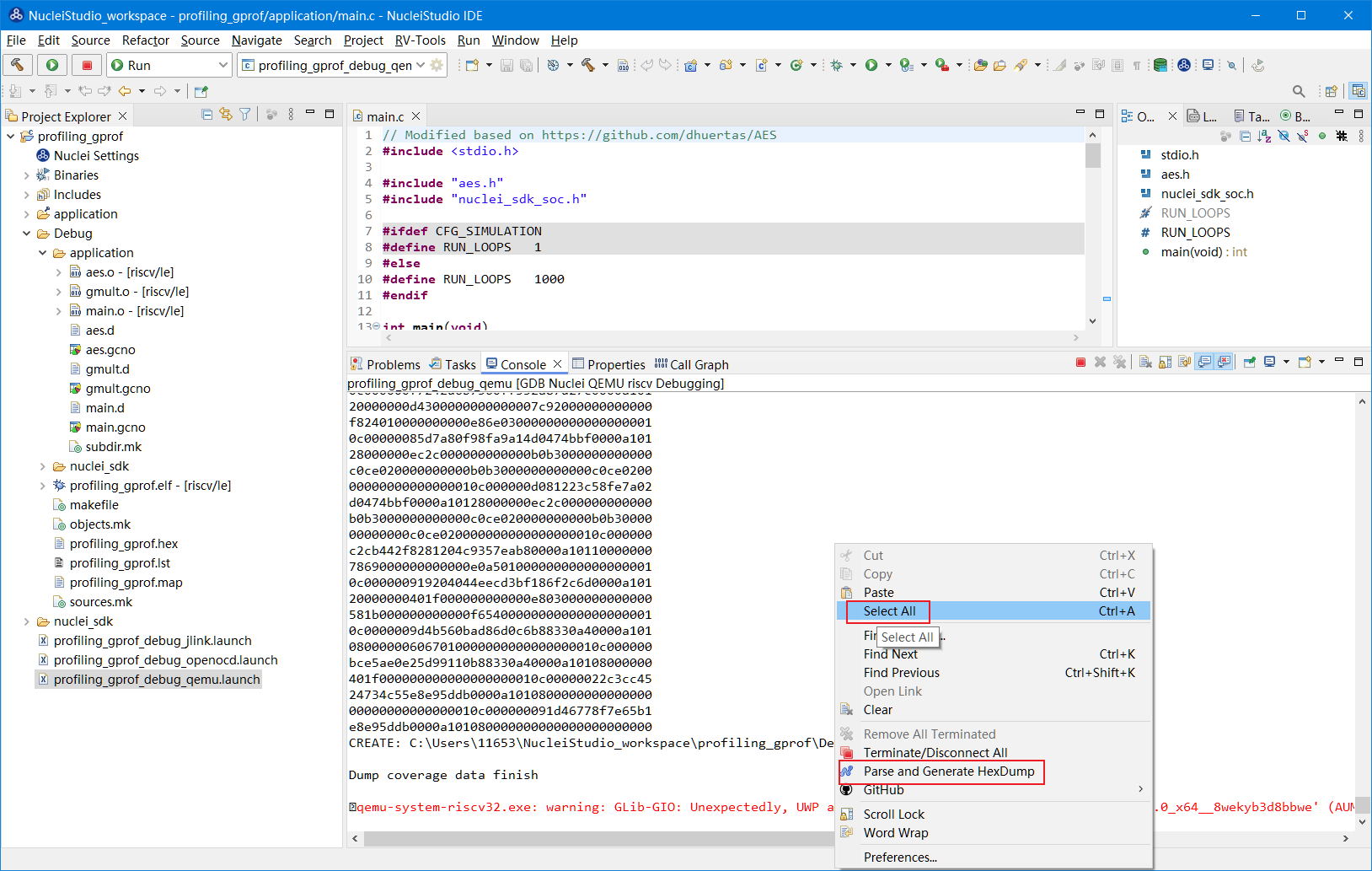
After the project is built, run it under QEMU or debug it on a real development board. This example runs the program under QEMU; the Profiling information is output in the Nuclei Studio Console window. When debugging on a development board, the Profiling information appears in the serial port output.

The output Profiling information must be parsed before Nuclei Studio can read it. Right-click in the Console window and select Select All from the context menu to select all output, then right-click again and select Parse and Generate HexDump.
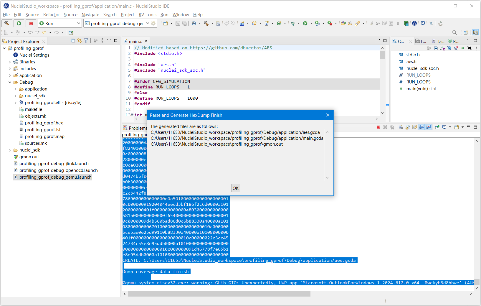
Nuclei Studio then analyzes the output and stores the results in the corresponding files.
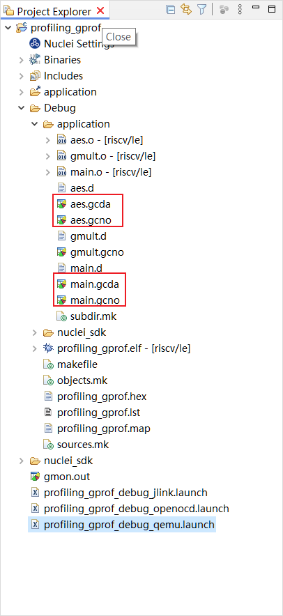
Check the Debug directory of the project again; the corresponding .gcda files have been produced.
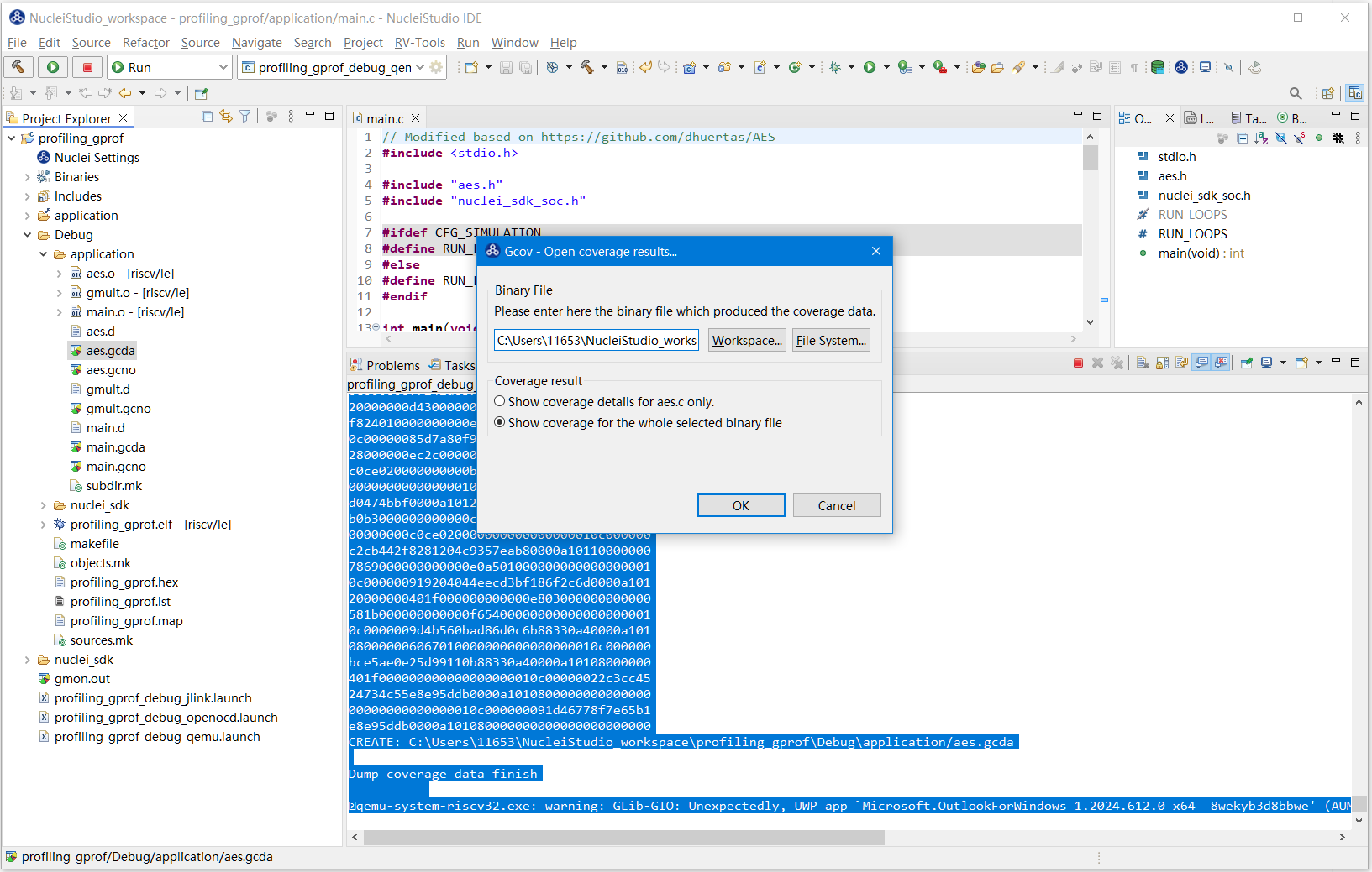
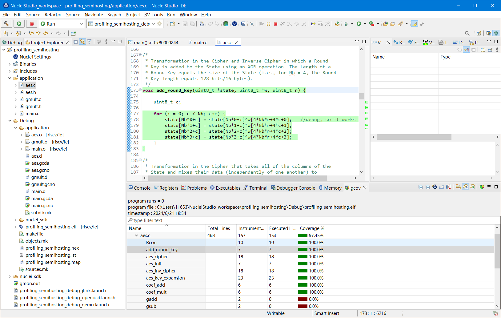
Double-click a .gcda file to open the Gcov tool and view the analysis results for the application. The results show whether each file or method was executed during program execution, as well as data such as the code execution coverage ratio.
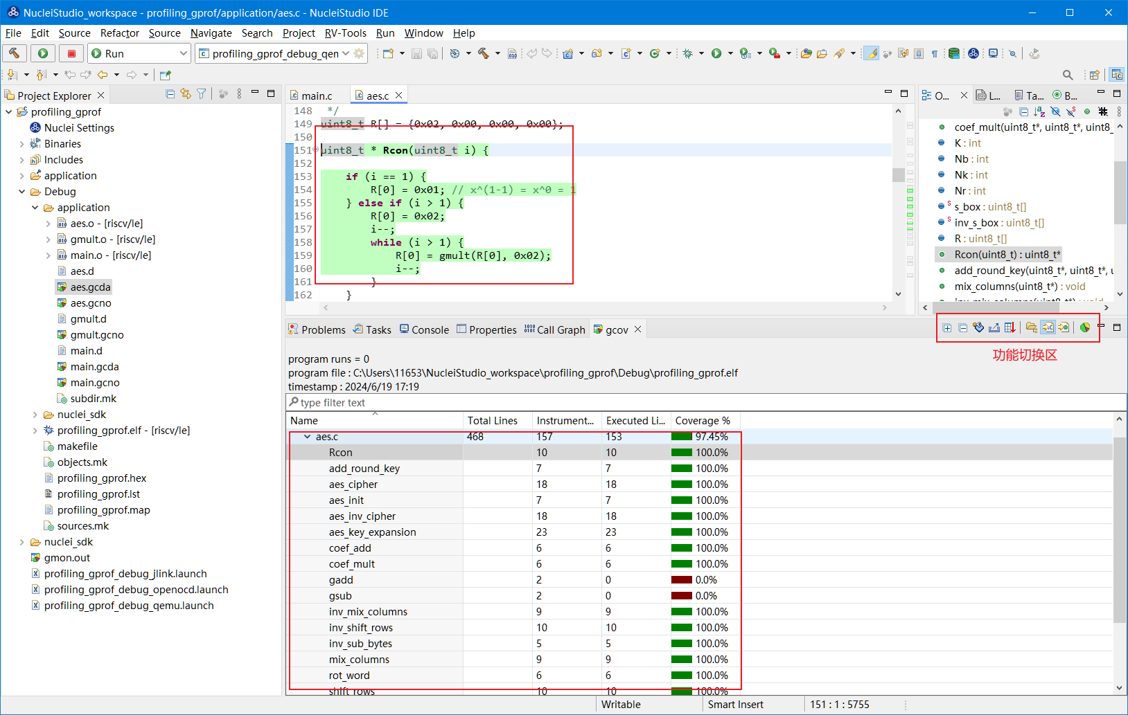
Double-click a row in Gcov, and Nuclei Studio automatically opens the corresponding file and colors its code: green indicates code that was executed during program execution, and red indicates code that was not. Use the Gcov results to optimize the code accordingly.
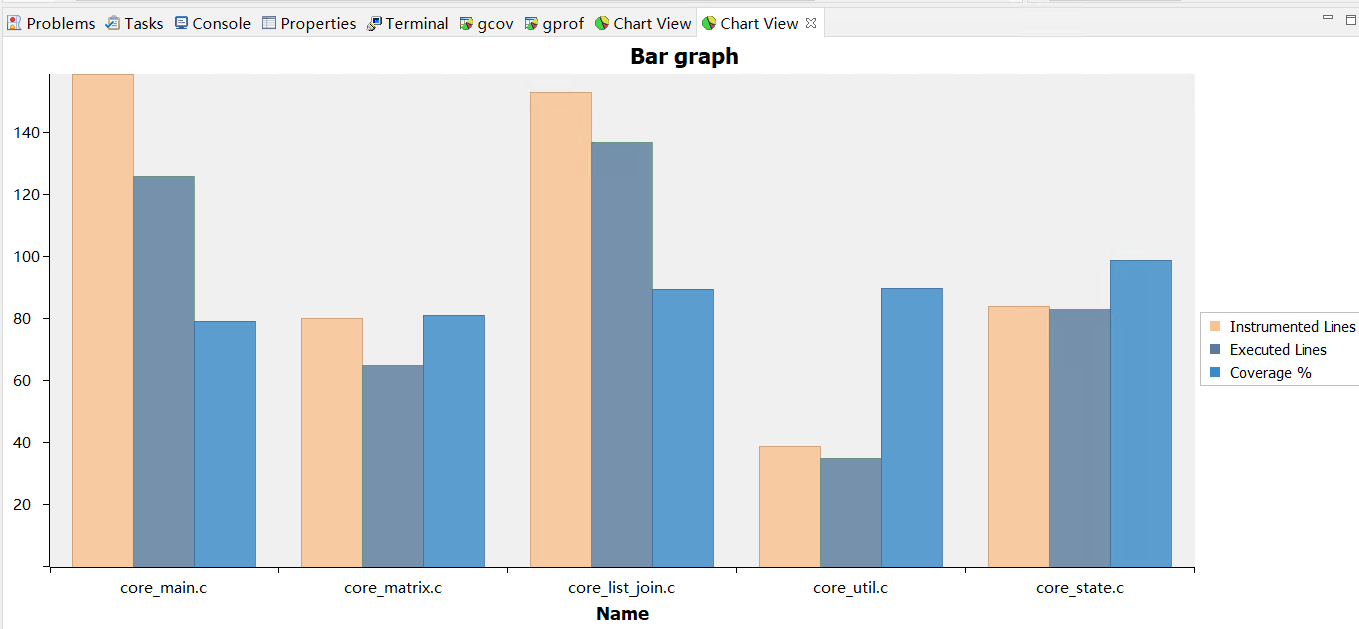
Code coverage also provides a histogram view of the data. Select the data item you want to view, click the histogram menu item, and configure it as needed.
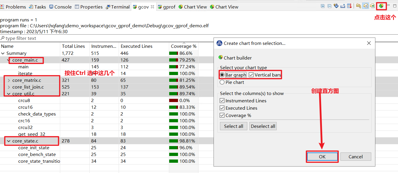
The code coverage histogram is then displayed in Nuclei Studio.
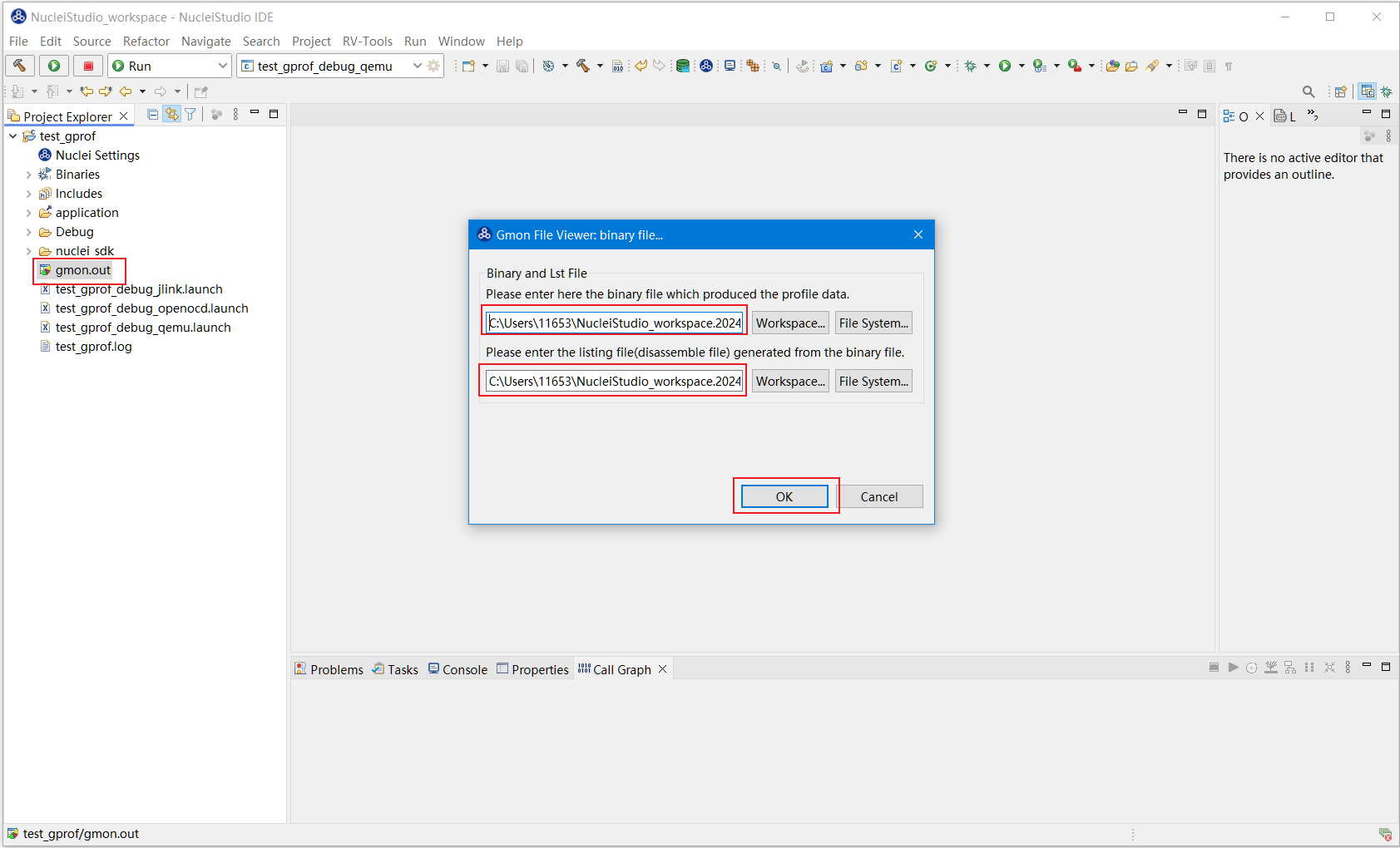
Double-click the gmon.out file. A file selection dialog pops up, prompting you to select the elf file and *.lst file related to the gmon.out file. By default, the elf file and *.lst file in the corresponding project are filled in automatically based on the current gmon.out. Click OK.
The Gprof tool starts and shows the analysis results for the application, including the call relationships of files and methods.
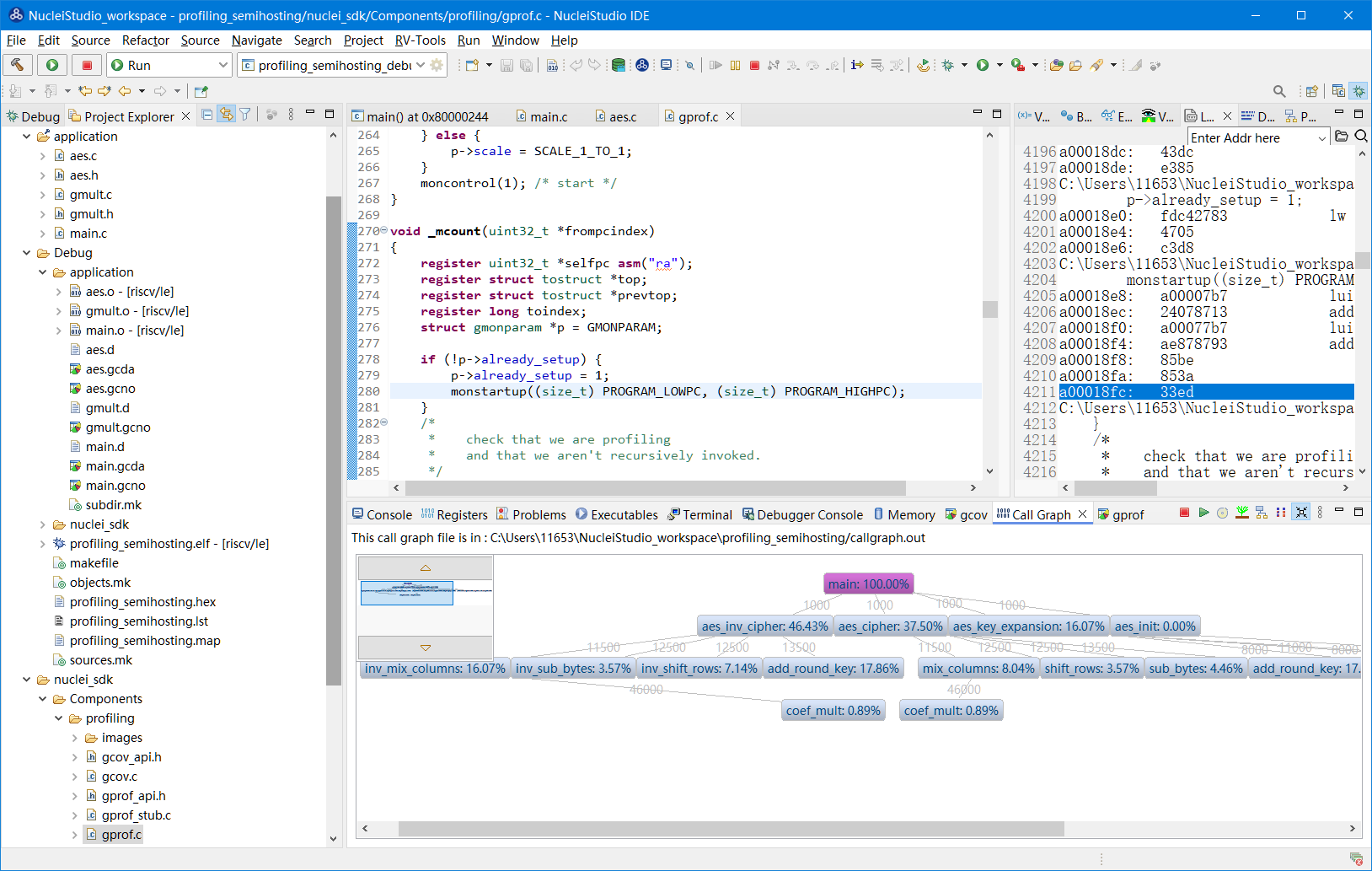
Double-click a row in Gprof, and Nuclei Studio automatically opens the corresponding source file at the corresponding line. It also opens the LST View tool and locates the line by addr, linking Gprof, the source code, and the disassembly code so you can quickly understand the program structure and call relationships.

Likewise, you can view a histogram of the profiling data in Nuclei Studio.

When Gprof is opened, Nuclei Studio parses the program’s call graph from the gmon.out file and generates a callgraph.out file. Double-click the callgraph.out file, or click the Open Call Graph View button in the Gprof toolbar, to start the Call Graph tool. For details on using Call Graph, see About Call Graph.

2.10.3.4.2. Using via Semihosting
After installing nuclei_sdk 0.6.0 in Nuclei Studio, create a Profiling demo to show how to use gprof and gcov test project, this time selecting Enable Semihosting. For details about the Profiling demo to show how to use gprof and gcov test project, see demo_profiling.
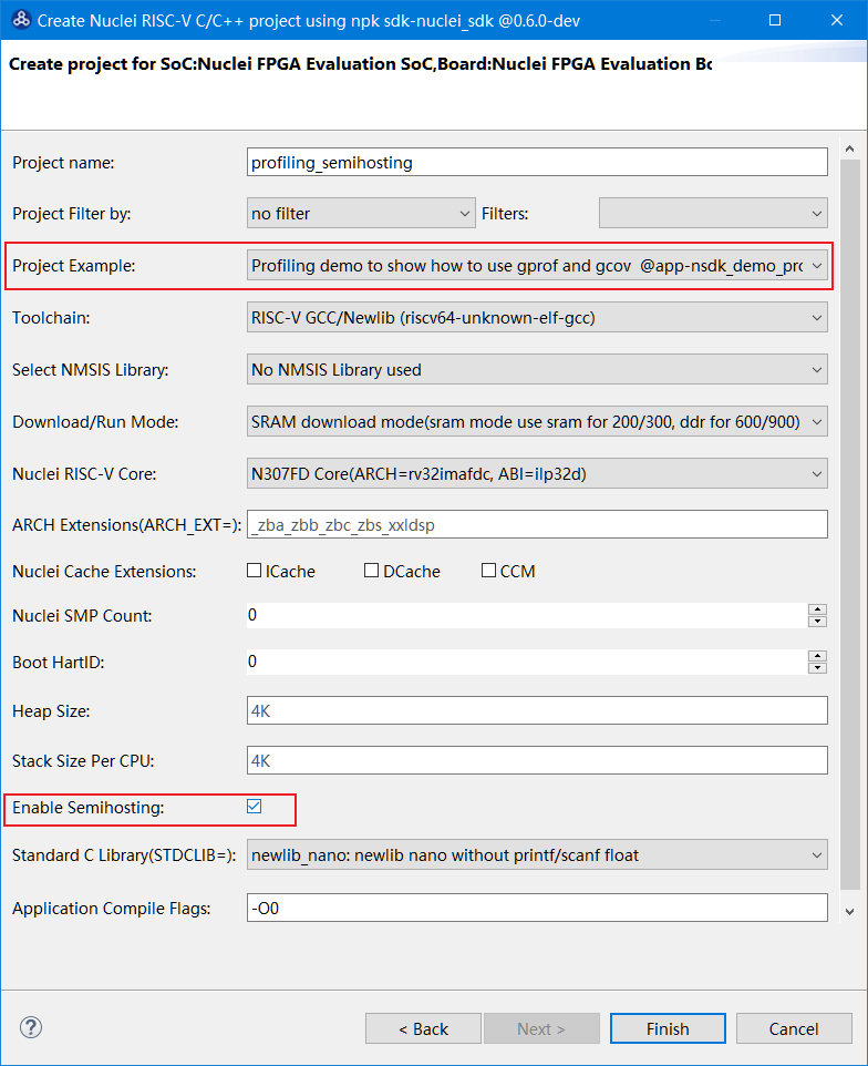
After the project is created, set the -pg --coverage compile option for the files or folders you want to analyze, then build the project.
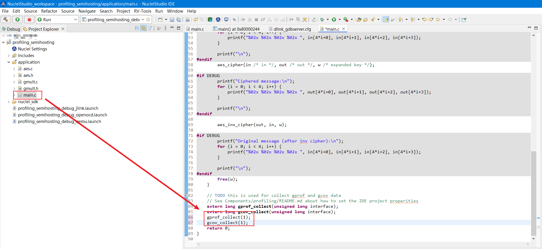
Also change gprof_collect(2); to gprof_collect(1); and gcov_collect(2); to gcov_collect(1); in the program (at the end of the main function in the test project). During execution, the results are then output as files through Semihosting.
Build the project. In the Debug directory of the successfully built project, you can see that several .gcno files have been generated.
After the project is built, run it under QEMU or debug it on a real development board.

This example runs the program under QEMU. After the program finishes running, refresh the project; several new files appear under the project: *.gcda files and *.out files. View the results as described above.
View the Code Coverage information of the application with the gcov tool in Nuclei Studio.
View the Profiling information of the application with the gprof tool in Nuclei Studio.

View the call relationship information with Call Graph in Nuclei Studio.
2.10.4. Using the Trace Feature
Trace is a powerful debugging technology that helps developers track and record key information during program execution, so they can effectively diagnose problems, optimize performance, and improve system stability.
Nuclei Studio integrates a Trace tool. Combined with the corresponding hardware and Nuclei OpenOCD, it lets you view Trace logs while debugging a project and troubleshoot problems together with the source code.
Note
The Nuclei System Technology WeChat Channel contains a video on How to Use the Trace Feature in Nuclei Studio. Search for the Nuclei System Technology WeChat Channel in WeChat to view it.
Note
For the Nuclei ETrace commands of OpenOCD, see the openocd.pdf manual under OpenOCD.
If you encounter any problems during use, check https://github.com/Nuclei-Software/nuclei-studio or submit an issue.
2.10.4.1. Trace UI Overview
Trace View
In Nuclei Studio, open the Show View dialog via Window->Show View->Other, find the RV Trace->Trace menu item, and click it to open the Trace view.

The Trace view consists of two parts: the Trace toolbar on top and the Trace record table below. The Trace toolbar provides the following items:
Trace setting
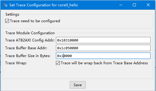
Opens the trace configuration, where you configure Trace ATB2AXI Config Addr, Trace Buffer Base Addr, Trace Buffer Size in Bytes, and Trace Wrap.
Start trace/stop trace
Starts or stops trace recording.
Trace clear
Clears all trace settings on the hardware.
Dump trace file
Dumps the trace file from the hardware.
Reload trace file
Reloads the contents of the trace record table locally.
Clear viewer
Clears the contents of the trace record table, as well as Trace Decode related configuration, such as the relationship between HartID and Thread.
Save trace log
Saves the trace record table as a CSV file.
Toggle instruction stepping
Opens the source code and disassembly code corresponding to the selected record.
Decode trace into flame
Parses flame graph information from the Trace records.
step into previous line
When a record is selected, jumps to the previous record and locates the corresponding source code and disassembly code.
step into next line
When a record is selected, jumps to the next record and locates the corresponding source code and assembly code.
Search for Addr
A search box for finding the trace record row with a given Addr.
search backward
Views the previous result when there are multiple search results.
search forward
Views the next result when there are multiple search results.
search exceptions or interruptions
Views the next result when there are multiple search results.
Page
Pagination controls. When there are many trace records, they are displayed across multiple pages for easier viewing.
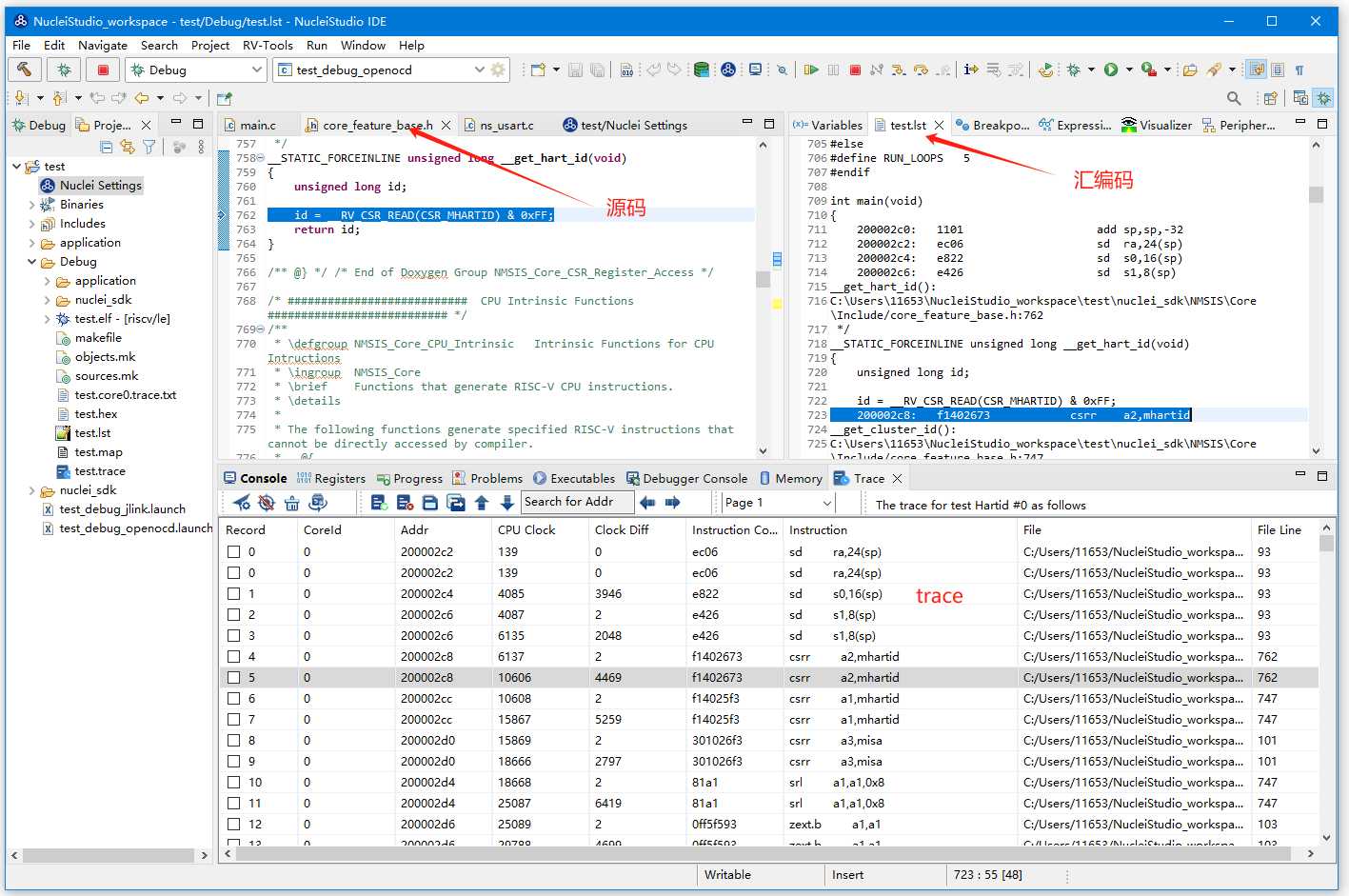
The Trace record table displays the records generated after Nuclei Studio decodes the dumped trace file. When you click a record, Nuclei Studio automatically locates the corresponding source code and disassembly code.
Record: record ID
CoreId: Core ID, mainly used to distinguish between different Cores in multi-core scenarios
Addr: instruction address
CPU Clock: clock cycle count
Clock Diff: clock cycle difference
Instruction Code: instruction code in hexadecimal
Instruction: instruction code
File: the file containing the source code corresponding to the instruction
File Line: the line number of the source code corresponding to the instruction
Trace Configuration
Here you can configure Trace ATB2AXI Config Addr, Trace Buffer Base Addr, Trace Buffer Size in Bytes, and Trace Wrap. The specific values depend on the hardware.
Check core support for Trace: If checked, the CPU is checked for Trace support before the Trace command is issued; if unchecked, the CPU support check is ignored when the Trace command is issued.
Trace need to be configured: Check this option if the Trace module must be configured. If it has already been configured elsewhere, do not check it. For example, in multi-core SMP/AMP scenarios the SoC has only one Trace module; if one core has already checked this option and configured the module, the other cores must not check it. Likewise, do not check it if the configuration has been done in C code or elsewhere.
Trace ATB2AXI Config Addr: Base address of the ATB2AXI module controller.
Trace Buffer Base Addr: The starting address where trace records are stored. For example, for a certain SoC: in flashxip mode, ilm (0x1c000000) is used as the buffer; in sramxip mode, dlm (0x08010000) is used as the buffer.
Trace Buffer Size in Bytes: The size of the buffer where trace records are stored, in bytes.
Trace Wrap: Whether automatic overwriting is allowed. If allowed, recording starts over from the beginning when the buffer is full.
Trace Decoder Configuration
In the Set Current Debug hart Configuration dialog, you can customize the following trace decoder parameters.
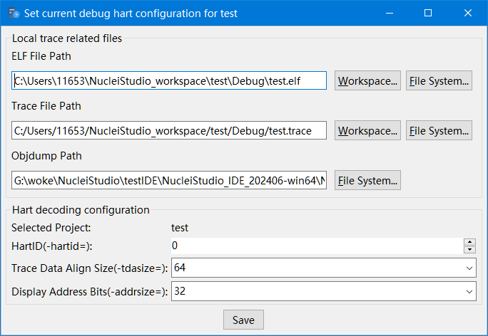
ELF File Path: The path of the elf file executed when the trace was produced.
Trace File Path: The path of the trace file to be parsed.
Objdump Path: The objdump tool is used during trace decode, so the path of the objdump tool must be specified here.
HartID: During trace decode, the HartID corresponding to the trace to be viewed must be specified. For single-core projects, the default is HartID=0.
Trace Data Align Size: The alignment size of the trace data, generally aligned with the hardware trace output width. The default values are 8, 32, and 64. If Trace Wrap is not checked, set this value to 8.
Display Address Bits: The number of address bits displayed after trace decode, generally 32, 64, or 128 bits.
Decode Mode: An extended trace decode feature. The default is 0.
Decode Limit: The limit on the number of trace decode entries, 5 million by default. The more entries, the higher the demands on your PC.
2.10.4.2. Using Trace
When using the trace feature, the Trace commands must be issued to the hardware through Nuclei OpenOCD or DLink while the project is being debugged. Currently, OpenOCD supports Trace recording in single-core, multi-core SMP, and multi-core AMP applications, while DLink only supports trace recording in single-core applications.
The following example uses OpenOCD to demonstrate the Trace feature.
2.10.4.2.1. Using Trace in a Single-Core Application
This document does not describe how to obtain the Nuclei-licensed CPU and the related supporting hardware or how to set up the hardware environment. Create the corresponding project and make sure it can run and debug on the hardware. The following example illustrates the process in a test environment we built ourselves.
In this example, we create a U900 single-core application named test from the demo timer template project and run it in FLASHXIP mode.
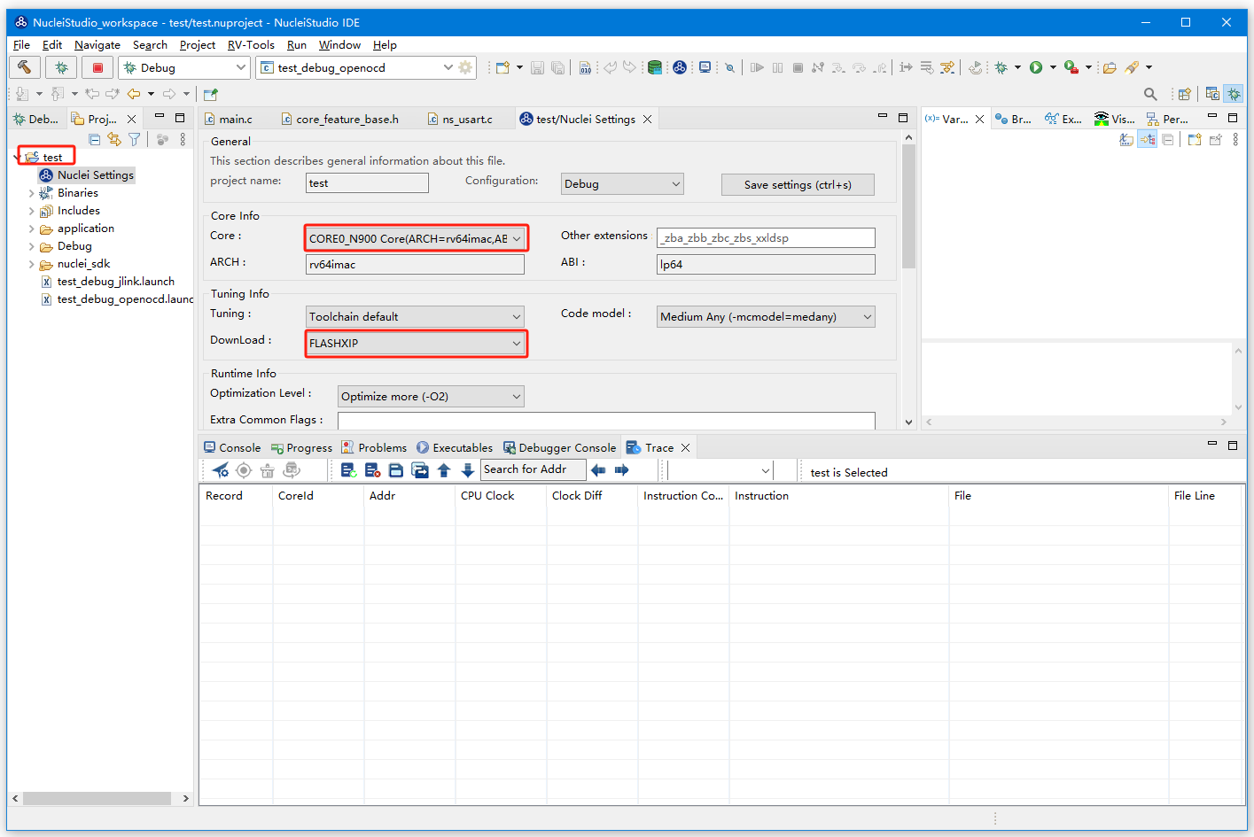
You can record the trace of the entire application run, or only the trace between two Debug breakpoints. After entering Debug mode, open the Trace view.

Open the Trace Configuration, configure the trace information, and click Save. If you do not want to save the configuration, close the window.
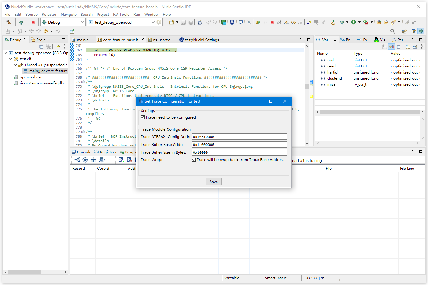
After Trace is configured, set two breakpoints, one as the Trace start point and one as the Trace end point. When the program stops at the start-point breakpoint, click the start trace button and continue debugging (such as stepping or running). When the program stops at the end-point breakpoint, click the stop trace button to end Trace.
This is only one way to use Start/Stop Trace; adapt it to your needs. When the trace ends (in multi-core scenarios, make sure Trace has ended on every CPU), click the Dump trace file button to download the trace file from the hardware to the local machine. By default, the downloaded trace file is stored in the debug directory under the project directory as <projectname>.trace.
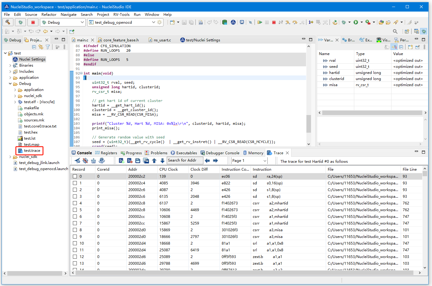
After the trace file is downloaded, Nuclei Studio pops up a Set current debug hart configuration dialog.
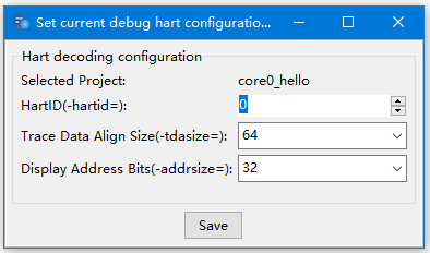
Fill in the correct information in the dialog (the HartID must be the hartid of the corresponding Thread) and confirm. Nuclei Studio then parses the trace file and generates the trace record table. Select any record in the table, and Nuclei Studio automatically finds the source code and disassembly code and locates the corresponding line (because the disassembly code and the source code open in the same view, move the disassembly code to another view yourself).
Note
Querying interrupts and exceptions is a new feature in Nuclei Studio 2025.10.
If a record in the Trace list contains an interrupt, the background color of that record turns green; if it contains an exception, the background color turns yellow. This helps you quickly distinguish interrupts from exceptions.
Click search exceptions or interruptions to view all interrupts or exceptions in the current project.
Double-click an interrupt or exception, and the Trace list automatically jumps to that record. Hover the mouse over the record to display its detailed information.
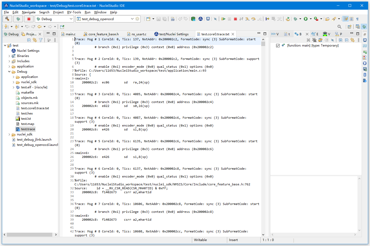
You can also double-click the <projectname>.trace file to view the trace file as text.
2.10.4.2.2. Using Trace in an SMP Multi-Core Application
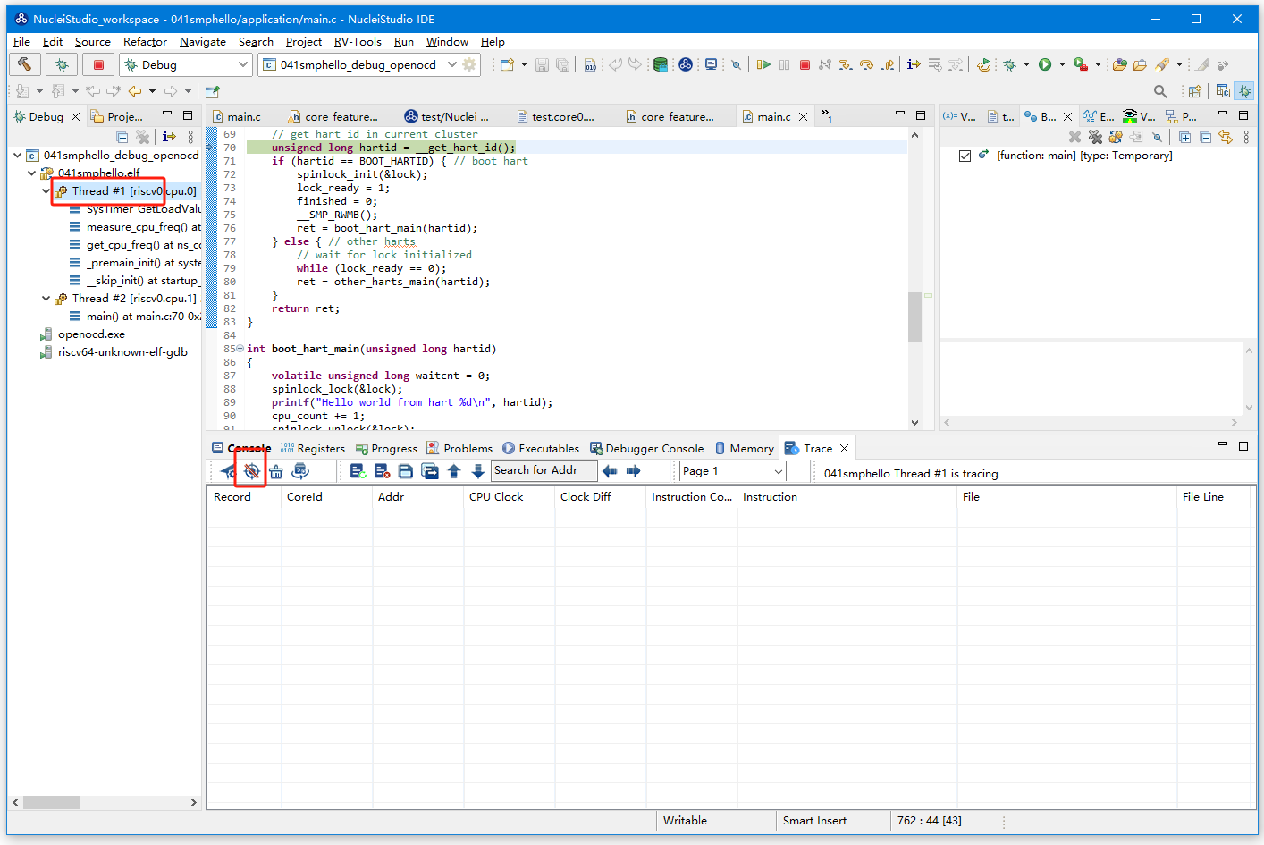
Using trace in an SMP multi-core application is similar to the single-core case. The difference is that in an SMP multi-core Debug session, all threads share one Trace Configuration, and you must select different Threads to start trace/stop trace for the individual CPU harts. In the Debug view, click a Thread, then click trace setting in the Trace toolbar to set up the Trace Configuration.

In the Debug view, switch between Cores by clicking different Threads. As shown below, clicking Thread #1 or the function name under Thread #1 selects Core 0 in the SMP multi-core application, and you can enable or disable Trace for Core
0. Once any Core has performed the start trace operation, the Trace Configuration is set in the hardware, and the other cores do not set it again when they perform start trace.
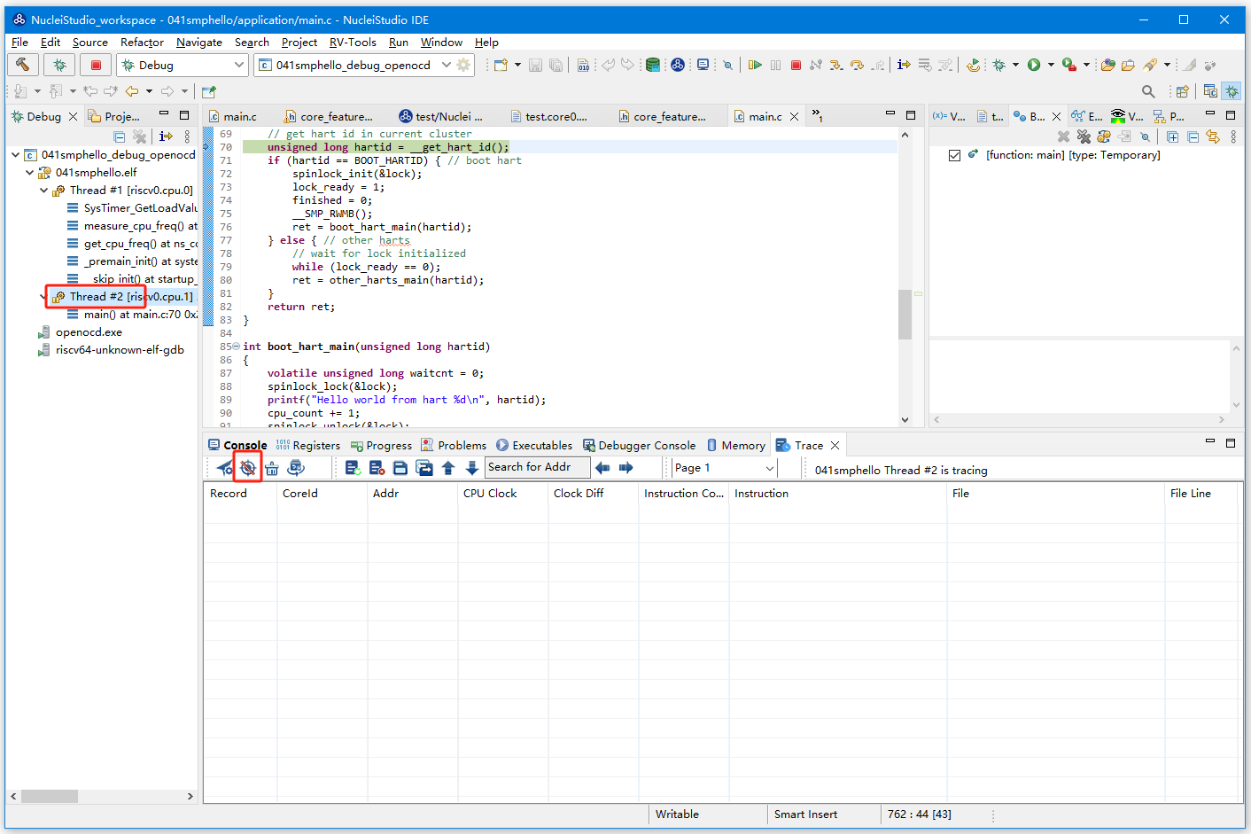
Similarly, click Thread #2 or the function name under Thread #2 in the Debug view to switch to Core 1 and perform the start trace/stop trace operations.
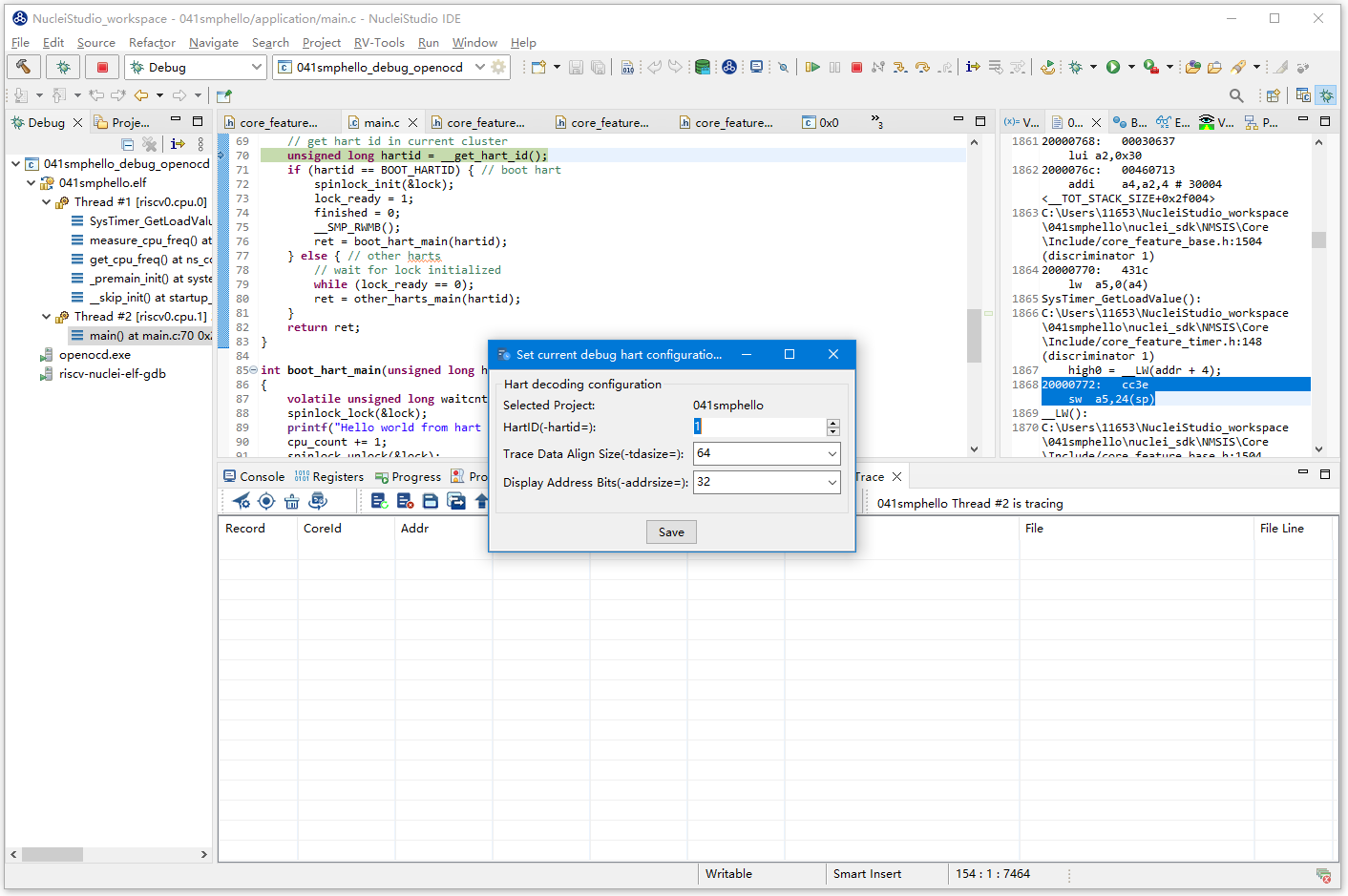
In an SMP multi-core application, the dump trace file command succeeds only after all Cores have performed stop trace. Only one copy of the Trace file needs to be downloaded. When decoding the trace file, set the Hart ID correctly to parse the trace record table for each core. As shown below, when HartID=0, you can view the Trace records corresponding to Core 0.

Similarly, when HartID=1, you can view the Trace records corresponding to Core 1.
2.10.4.2.3. Using Trace in an AMP Multi-Core Application
Using trace in an AMP multi-core application is also similar, and the trace configuration is shared as well: different threads share one trace configuration, but you can start trace/stop trace for each core individually through its thread. As shown below, in the Debug view, click Thread #1 or the function name under Thread #1 to switch to Core 0 in the AMP multi-core application, then click trace setting in the Trace toolbar to set up the Trace Configuration for Core 0.
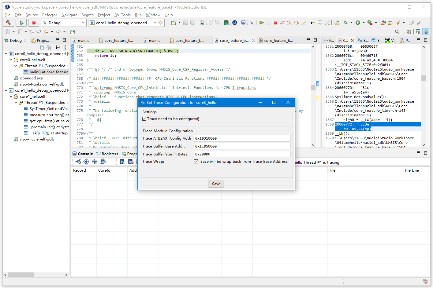
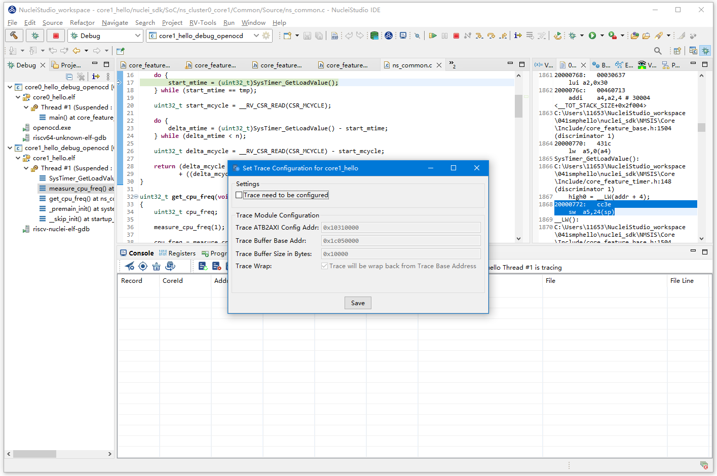
In the Debug view, click Thread #2 or the function name under Thread #2 to switch to Core 1 in the AMP multi-core application, then click trace setting in the Trace toolbar to set up the Trace Configuration for Core 1. Because the trace configuration is shared in an AMP multi-core application, uncheck Trace need to be configured here so that the trace feature is used without applying new settings.
After the Trace Configuration is set, switch between Cores through the Threads in the Debug view to perform the start trace/stop trace/dump trace file operations. Note that the Core for which the Trace Configuration is set must start trace first, so that the configuration is written to the hardware; only then can the other Cores perform the start trace/stop trace/dump trace file operations normally.
In an AMP multi-core application, make sure all Cores have performed stop trace before executing dump trace file. Otherwise, one Core may dump the trace file while the other Cores are still recording, and the resulting Trace file will not match expectations. Each project application must dump its own copy of the trace file, although the contents of the dumped files are identical. When decoding the trace file, also set the Core Hart ID correctly so that the corresponding trace record table can be parsed. The remaining operations are the same as described above.
2.10.4.2.4. Viewing Offline Trace
If you have obtained a trace file through the command line or other means, open Set Current Debug hart Configuration, configure the parameters as required, and the trace tool in Nuclei Studio parses the trace file.
2.10.4.3. Using Flame View with Trace
Note
In Nuclei Studio 2025.10, we introduced the Flame View feature, which clearly presents the call stack and time consumption during program execution through a visual flame graph, enabling developers to analyze performance hotspots more efficiently and accelerate troubleshooting.
Trace inherently records the program execution process, so it is well suited for parsing into a flame graph. Assuming you have already obtained the <projectname>.trace file, click the Decode trace into flame button.
If the <projectname>.trace file has not been parsed yet, the Trace parsing configuration page pops up first (see the previous sections for the configuration items). Complete the configuration and click Decode to start parsing.
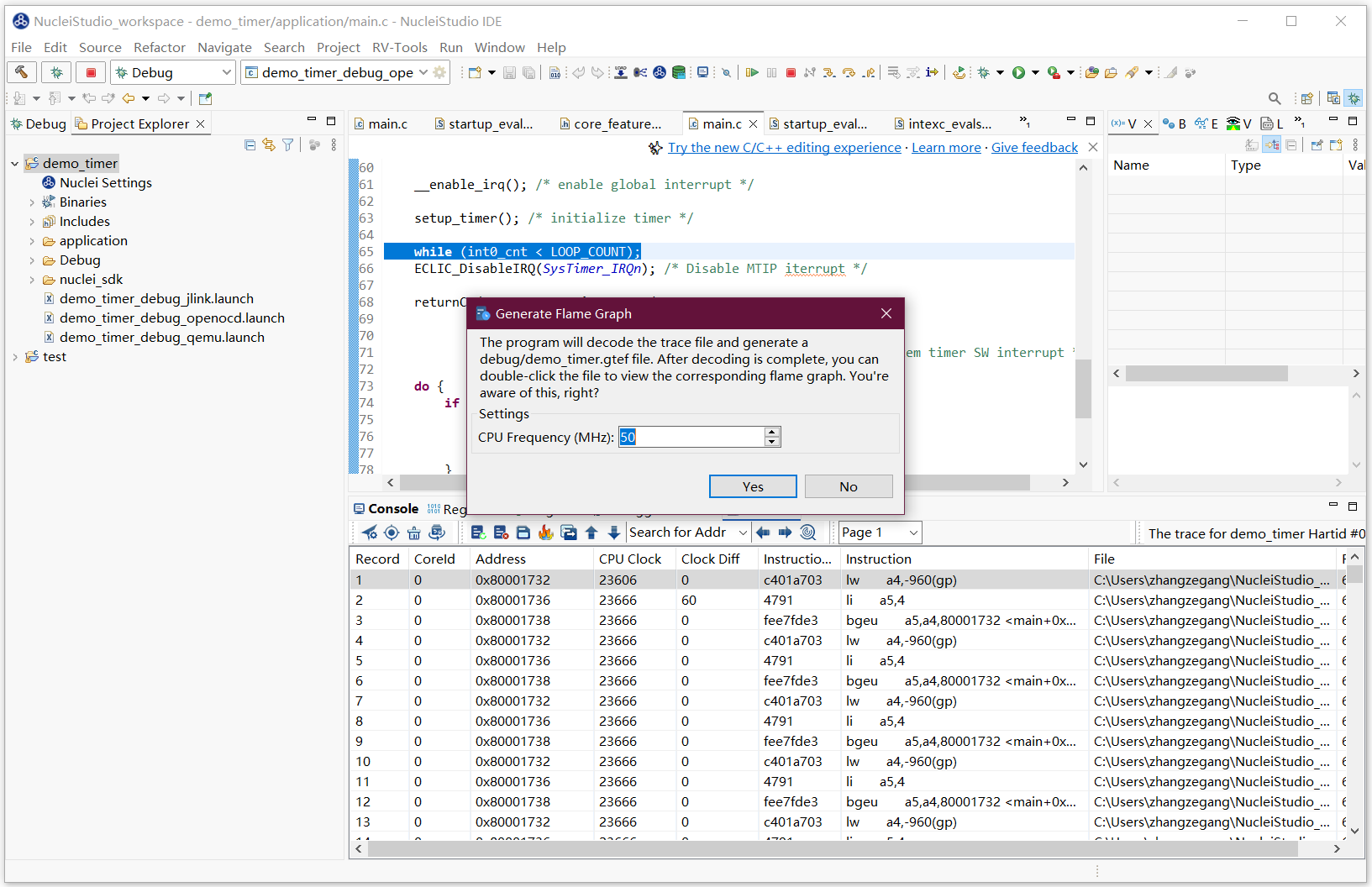
At the same time, the IDE opens the Flame View import wizard, which prompts that the corresponding <projectname>.trace file is about to be generated. Once the file is generated, double-click it to import it into Flame View for visual analysis. The wizard asks you to enter the current CPU operating frequency (for example, 50 MHz in this test) so that the timing information can be restored accurately.

If the <projectname>.trace file has already been parsed, the corresponding trace data is extracted directly from the existing Trace list, and the Flame View import wizard pops up immediately, skipping the repeated parsing step.
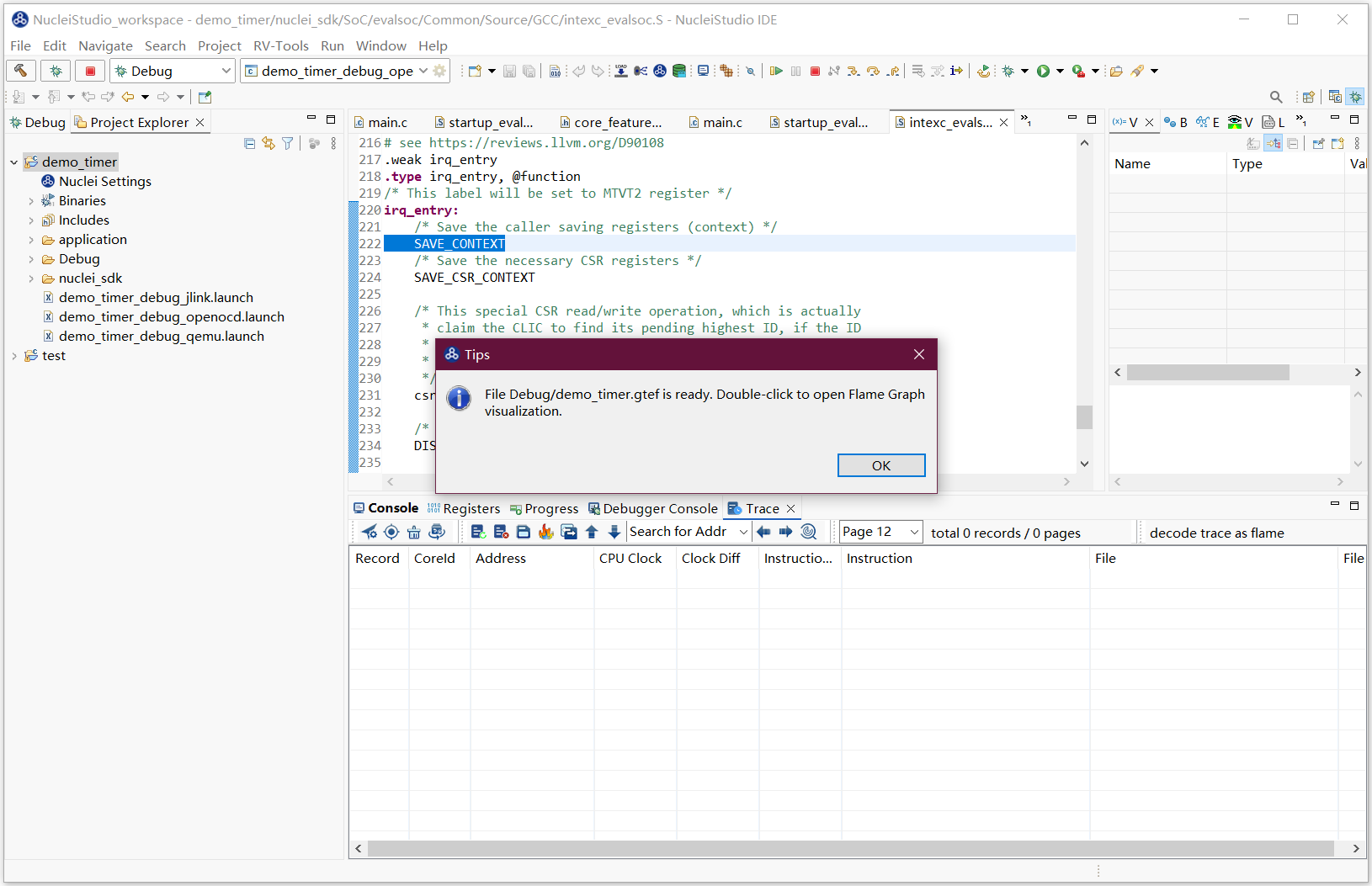
After the Trace list is parsed and the <projectname>.gtef file is generated, the IDE automatically prompts that the operation is complete.
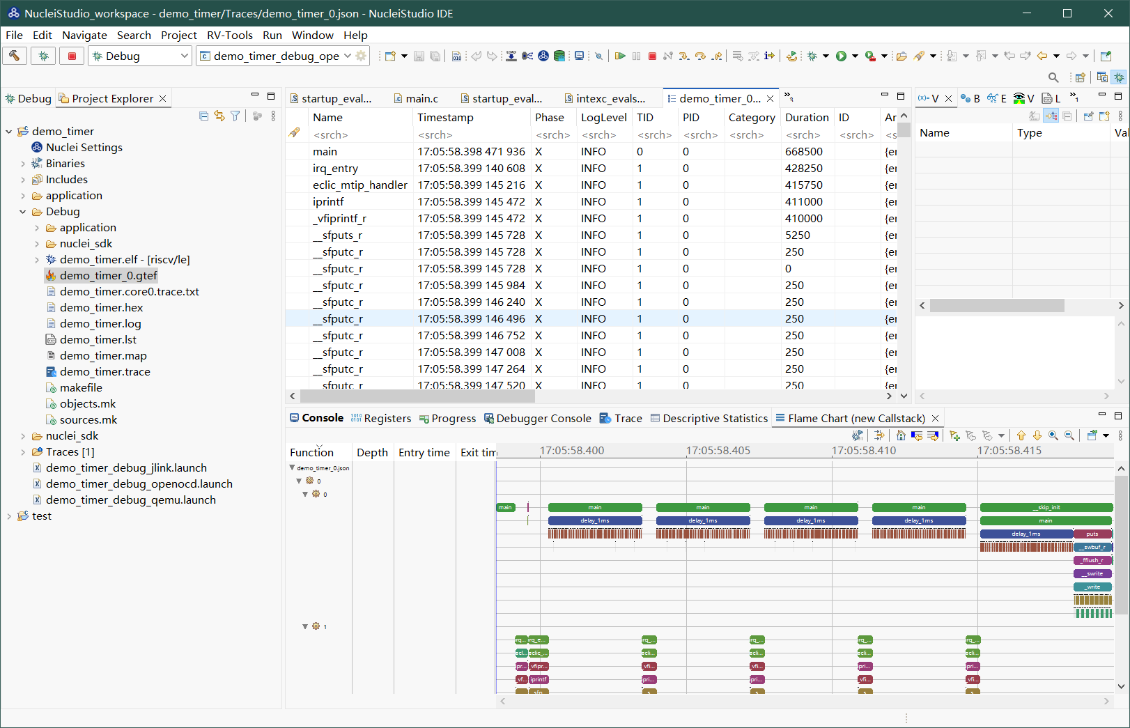
A <projectname>.gtef file now exists in the Debug directory. Double-click the file to view the flame graph of the project. Note: if the <projectname>.gtef file is updated, double-click the file again to re-import it into Flame View. For details about the Flame View feature, see Using Flame View.
2.10.5. Using RVProf
Note
Starting with Nuclei Studio 2025.10, the RVProf feature is supported on Windows, with the same usage as on Linux.
RVProf is a performance analysis tool developed by Nuclei System Technology for the CPU cycle model. Nuclei Studio has supported RVProf since version 2024.02.dev. Using RVProf involves three steps: the Cycle model tool runs the code and produces a .rvtrace file; the RVProf tool parses the .rvtrace file into a .json file; and Google’s open-source Perfetto Trace Viewer parses and displays the .json file. Because the CPU cycle model is currently only available for Linux, this document demonstrates the feature in a Linux environment.
If you encounter any problems during use, check https://github.com/Nuclei-Software/nuclei-studio or submit an issue.
2.10.5.1. Test Environment
The CPU cycle model places high demands on the hardware at runtime. It runs better on systems with four or more cores, and using it in a virtual machine is generally not recommended. For a better experience, this test was performed on a workstation.
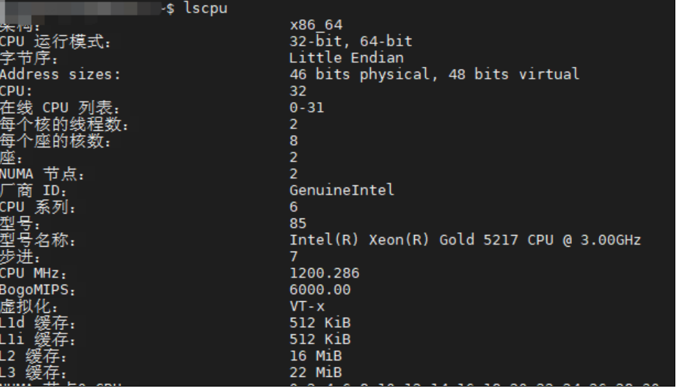
2.10.5.1.1. Preparing the Test NPK Packages
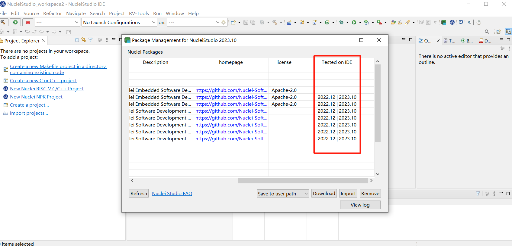
Currently, this feature requires test packages in Nuclei Package (NPK) format. Install the related packages into Nuclei Studio; for the installation procedure, see the NPK package sections of the Nuclei Studio manual. Because the RVProf test packages are not public, contact us to obtain them.
cymodel.zip: the NPK Tools package for cymodel
rvprof.zip: the NPK Tools package for RVProf
Rvprof helloworld.zip: the test demo NPK App package
2.10.5.1.2. Creating the RVProf Test Project
Before creating a project, check in Nuclei Package Management that the NPKs are installed correctly. Because the test demo depends on nuclei_sdk, sdk-nuclei_sdk must also be installed first, as shown below:
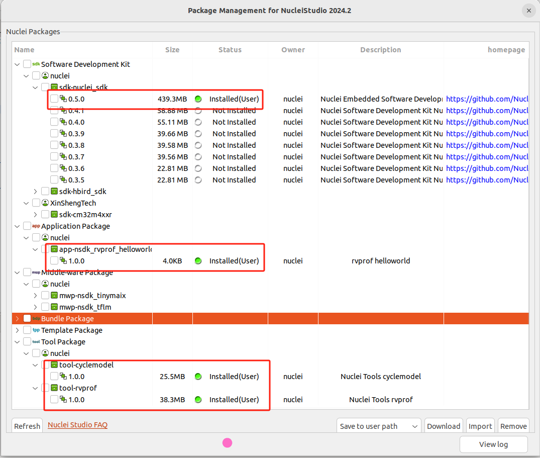
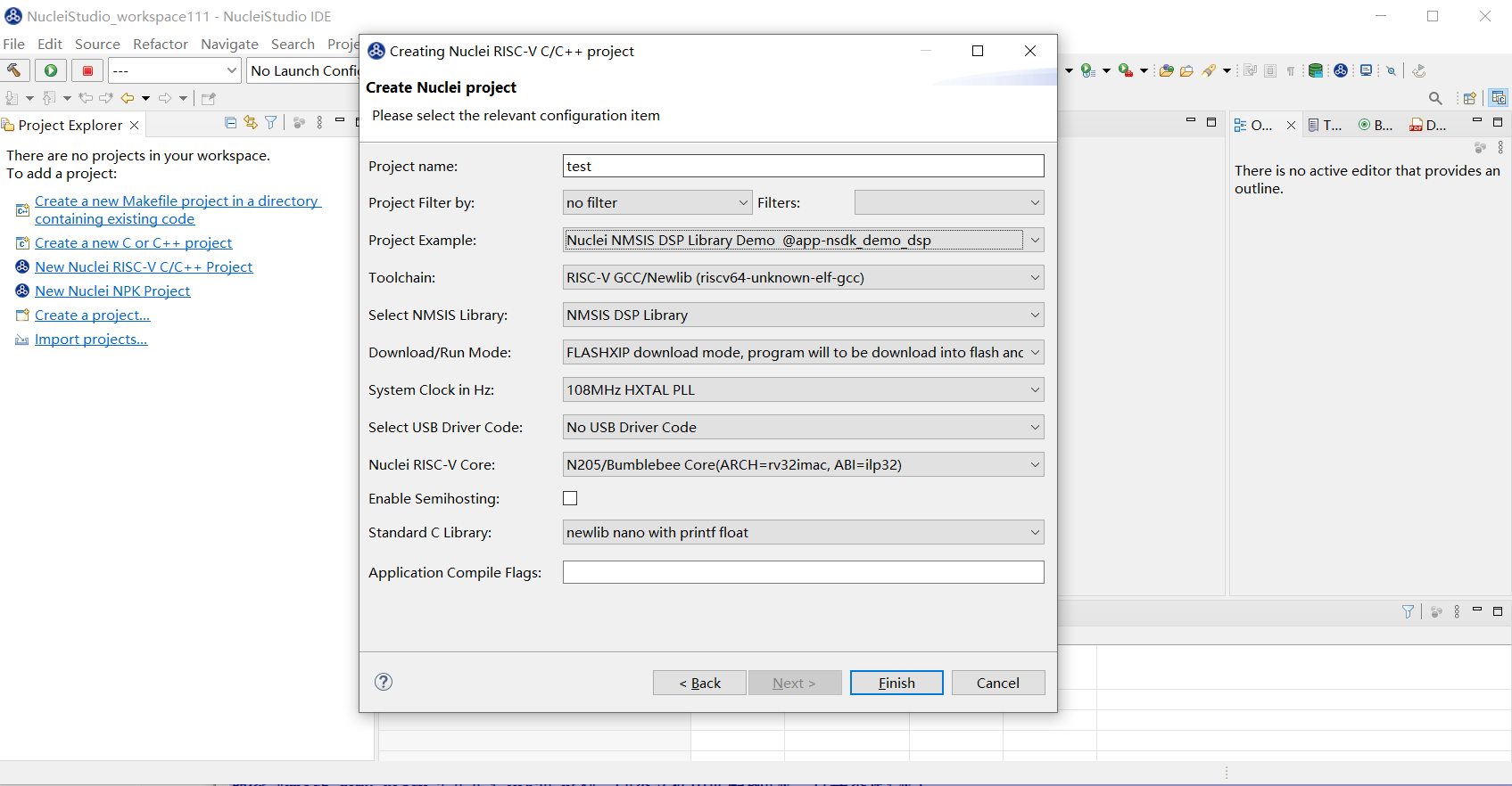
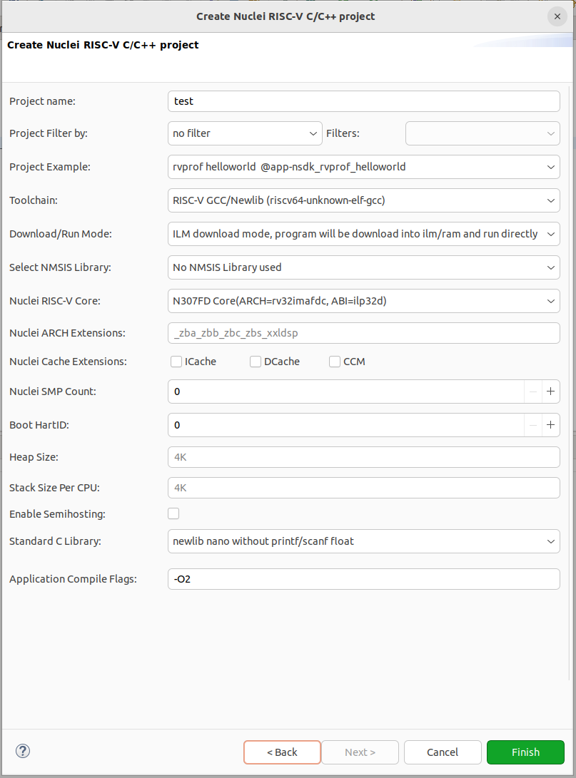
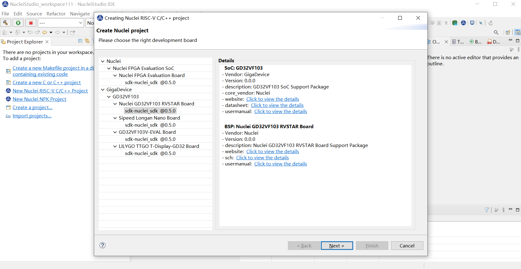
Then create a test project. In the project creation wizard, go through New Nuclei RISC-V C/C++ Project -> sdk-nuclei_sdk@0.5.0 -> next. On the project configuration page, enter the project name, select Project Example rvprof helloworld@app-nsdkrvprof_helloworld, and set Nuclei RISC-V Core to N307FD (the core must match the CPU cycle model).
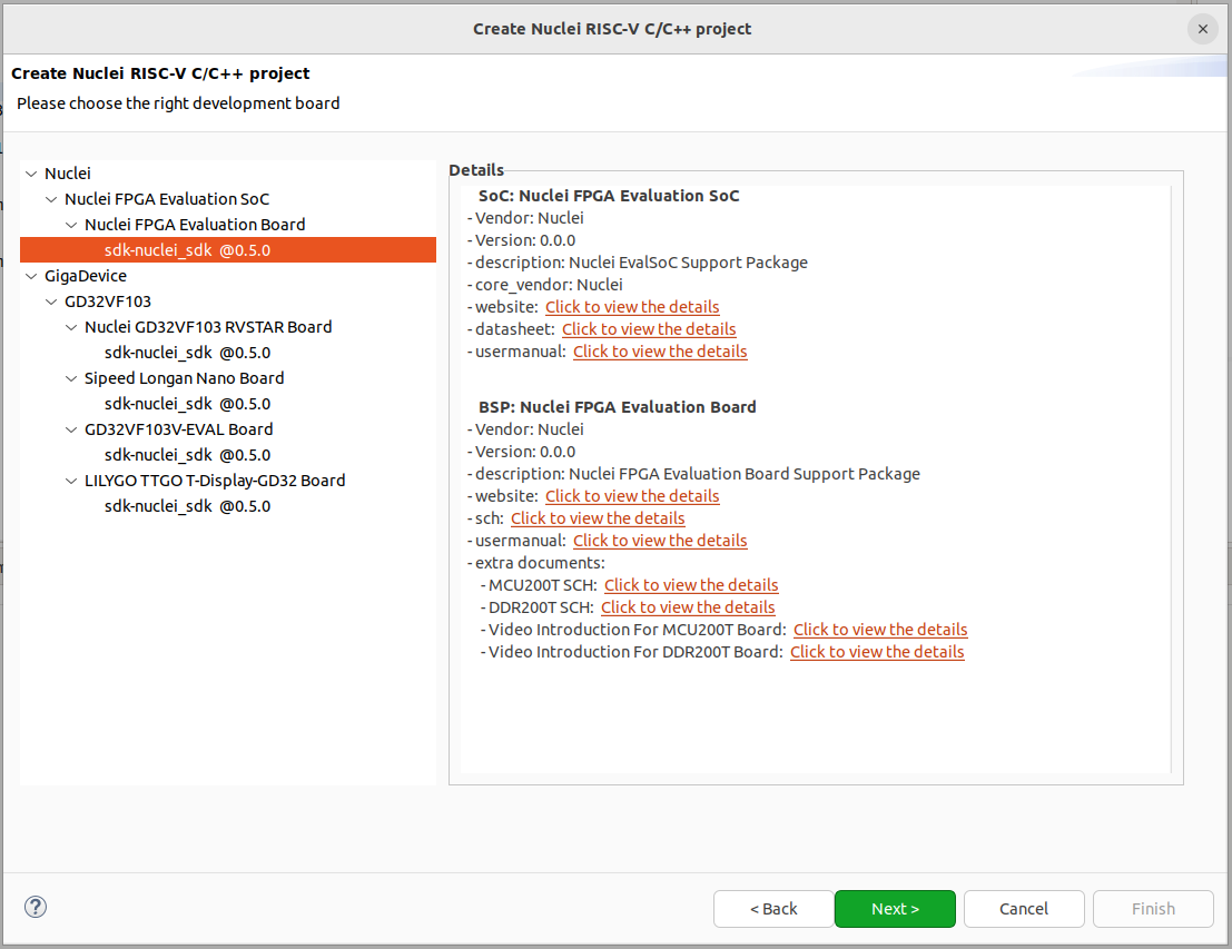
Under Project Example, select the Rvprof helloworld project from the imported demo NPK App, then click Next to complete the project creation.
The created test project contains an additional test_debug_rvprof.launch file with the RVProf configuration, as shown below. The Cycle Model timeout value sets the Cycle Model timeout. Because Cycle Model takes a long time to run, set a short timeout for a relatively simple project so that the Cycle Model run is interrupted promptly when the time is up. The timeout in RVProf serves a similar purpose.

2.10.5.2. Viewing the RVProf Results
After the project is created, select test_debug_rvprof.launch in the Launch Bar and click the run button in the toolbar. Nuclei Studio then completes the following tasks in sequence and displays the final results in Perfetto Trace Viewer.
Build the project code
Start Cycle Model and produce the trace file
Start RVProf to parse the trace file and generate the json file
Start Perfetto Trace Viewer to display the results
Cycle Model startup and log output
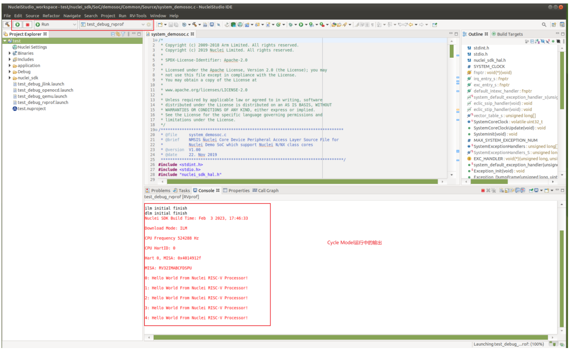
perfetto starting the local service

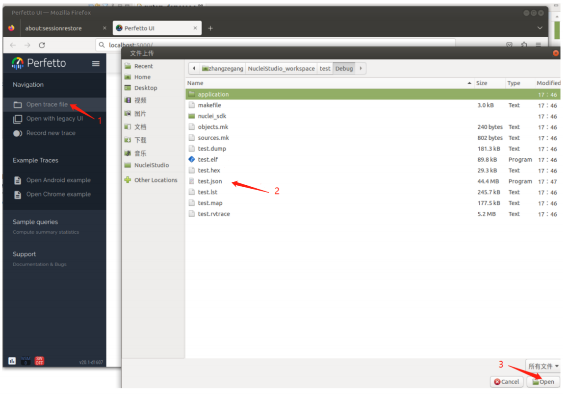
The official address of Perfetto Trace Viewer is https://ui.perfetto.dev/. By default, Nuclei Studio tries to open https://ui.perfetto.dev/ and automatically loads and parses the json file. If the site cannot be opened due to network issues (it is an overseas server), Nuclei Studio starts a local Perfetto Trace Viewer service and automatically opens localhost:5000/. In this case, manually load the Debug/test.json file under the project directory. The trace results are then displayed in Perfetto Trace Viewer.
Nuclei Studio starts a web service locally and opens Perfetto Trace Viewer at the same time.

Click Open trace file, locate the json file generated in the project, and load it manually into Perfetto Trace Viewer.
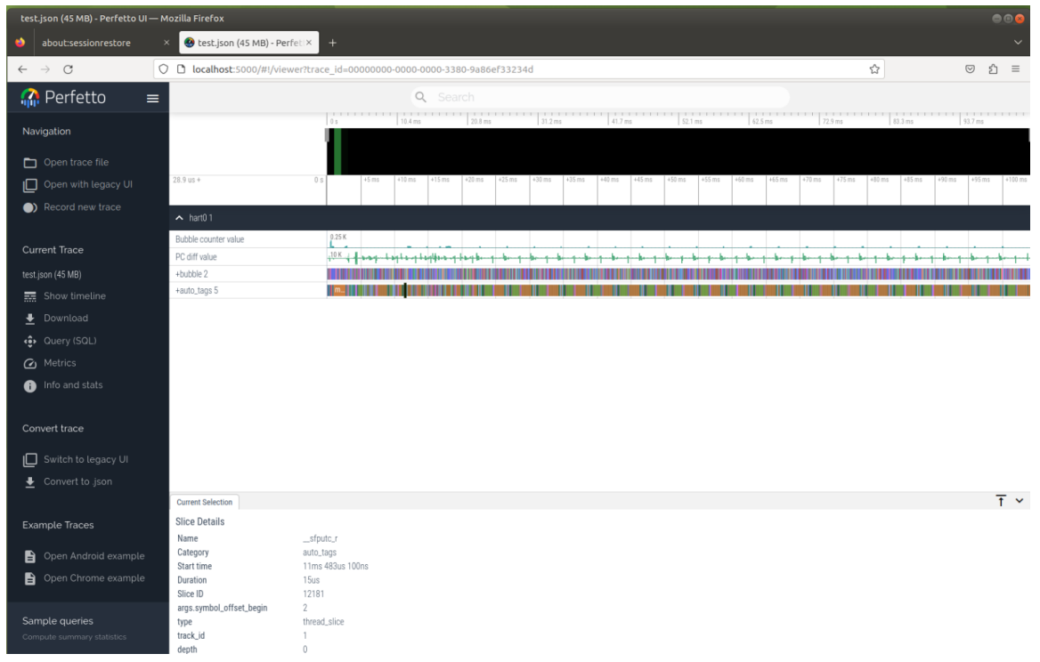
You can now view the RVProf trace results in Perfetto Trace Viewer. Use the W/A/S/D keys to navigate and view more detailed information.
2.10.6. Nuclei NICE Wizard
Note
The Nuclei System Technology WeChat Channel contains a video on Nuclei NICE Wizard. Search for the Nuclei System Technology WeChat Channel in WeChat to view it.
Nuclei NICE Wizard is a tool integrated into Nuclei Studio that simplifies and accelerates the creation of NICE (custom instruction extensions) and VNICE (vectorized custom instruction extensions) instructions. Through a graphical interface, you can quickly configure custom instructions and generate the required code framework, enabling hardware acceleration of specific application algorithms:
Simplified development process: reduces the time from concept to implementation of custom instructions.
Improved efficiency: improves the execution efficiency of applications by generating optimized instruction code.
Easy integration: the generated code can be integrated directly into existing projects.
2.10.6.1. Creating a .nice File and Opening Nuclei NICE Wizard
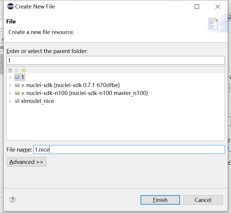
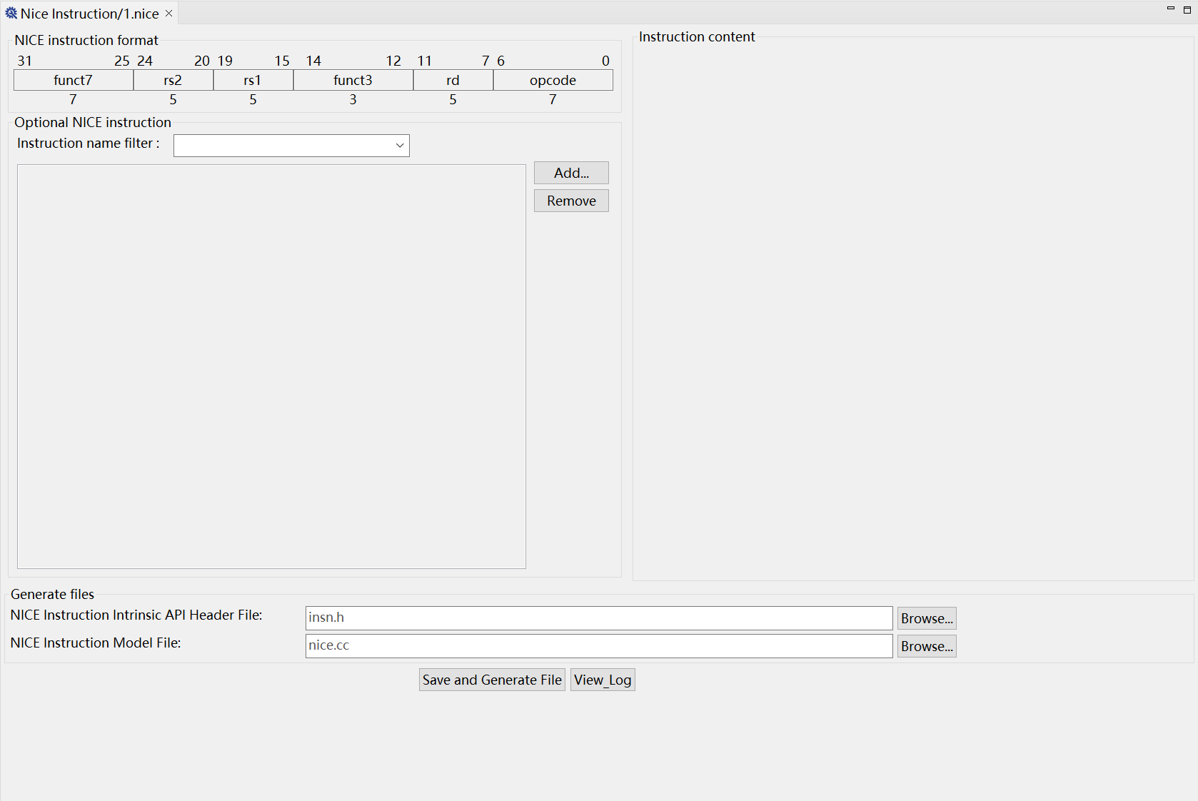
Open the target project in Nuclei Studio, create a *.nice file (for example aicc.nice) in the project root directory, and double-click it to open Nuclei NICE Wizard.
2.10.6.2. Adding an Instruction
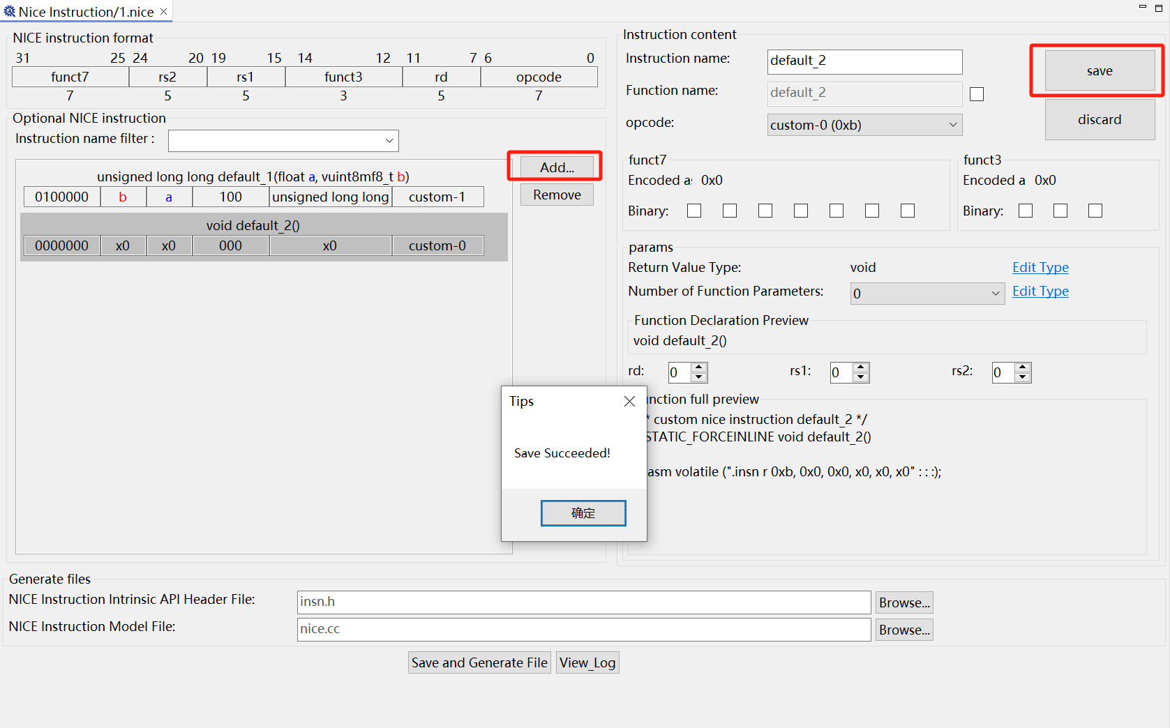
Click Add..., modify the instruction content as needed, and click save in the upper right corner.
The following example creates two instructions. The instruction selected on the left turns gray, and its content is displayed on the right.
2.10.6.3. Deleting an Instruction
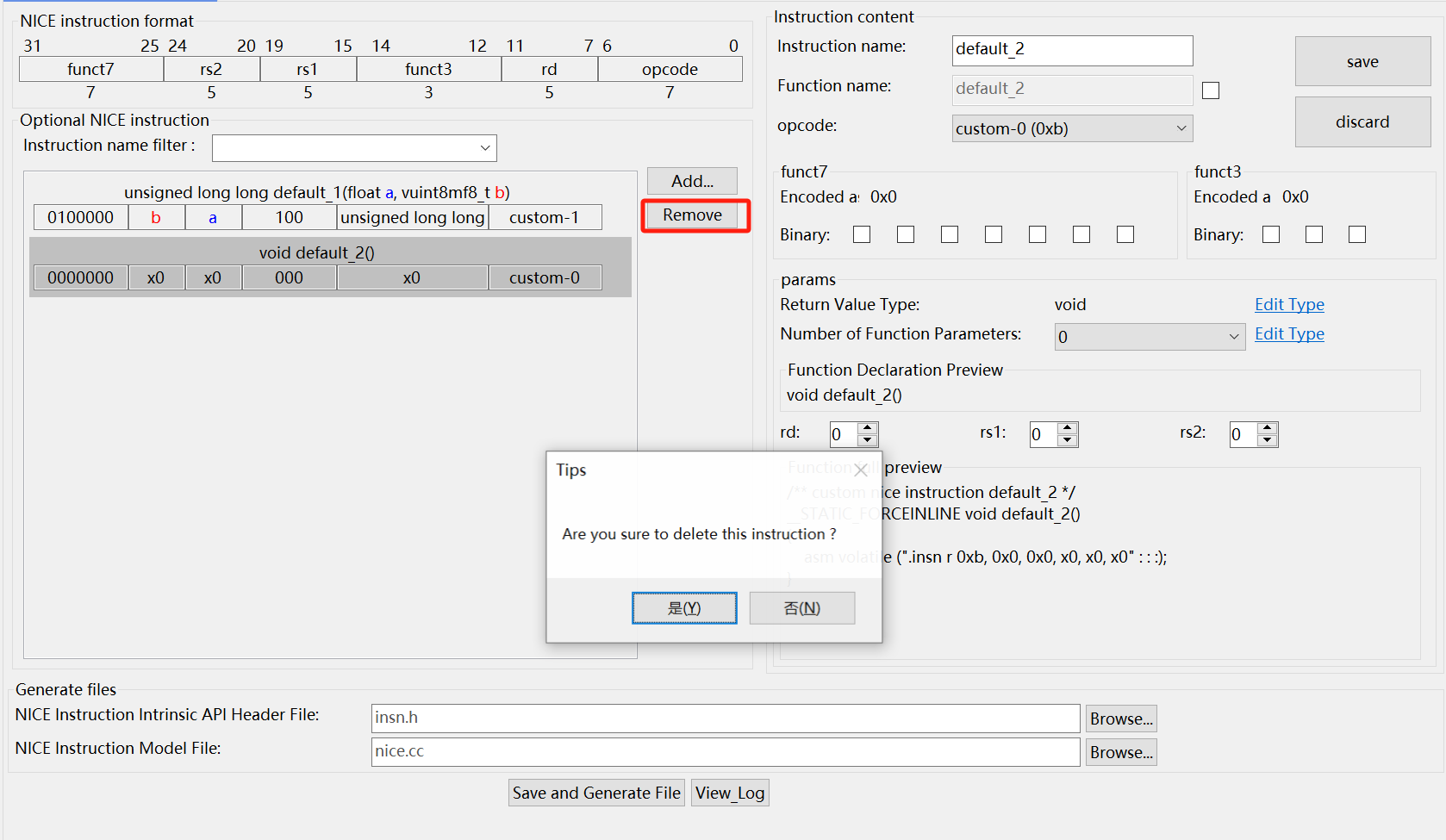
Select the instruction on the left, click Remove, and confirm the deletion.
2.10.6.4. Modifying an Instruction
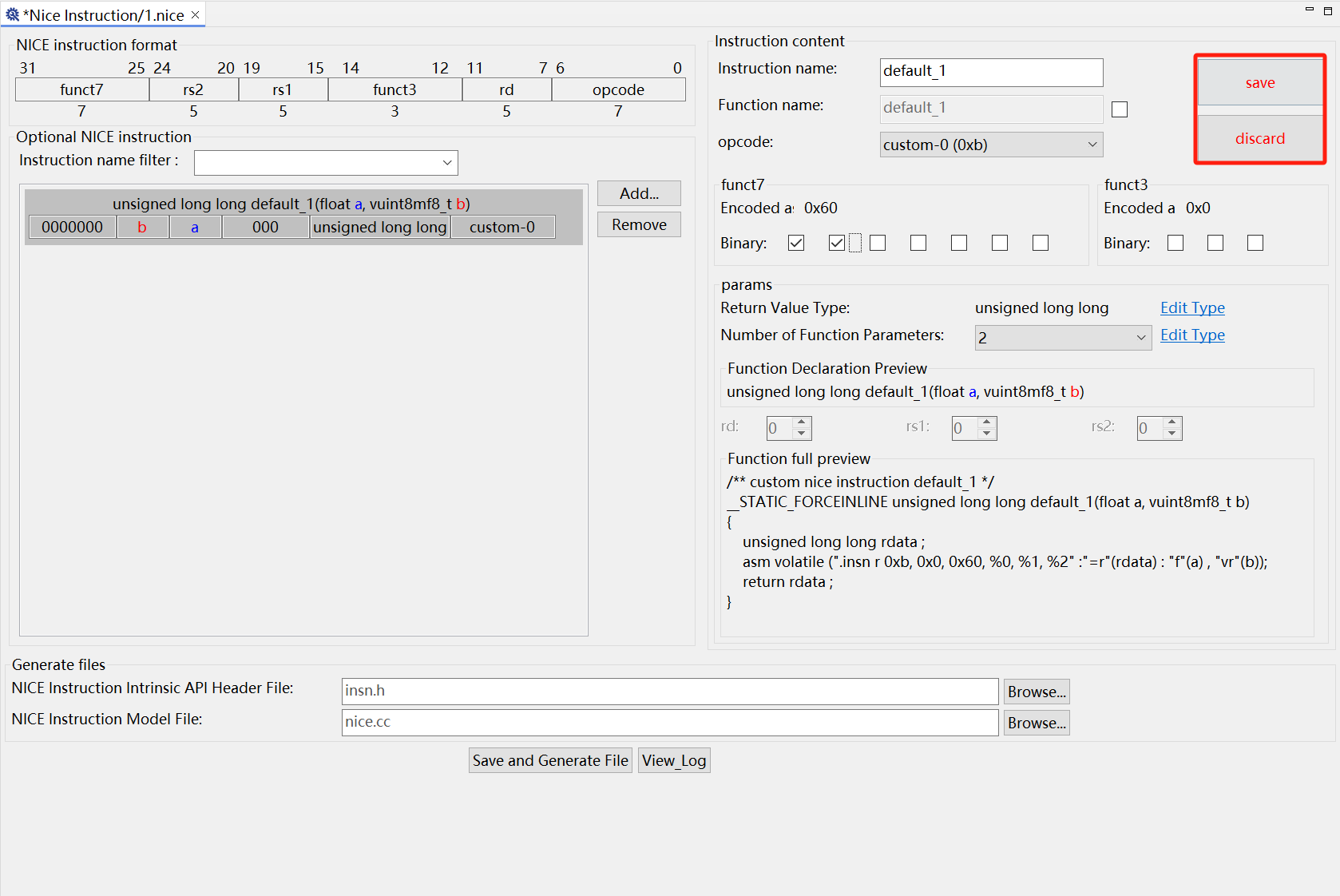
Select the instruction on the left. After you modify the instruction content, the save and discard buttons in the upper right corner turn red; click them to save or discard the changes.
2.10.6.5. File Generation
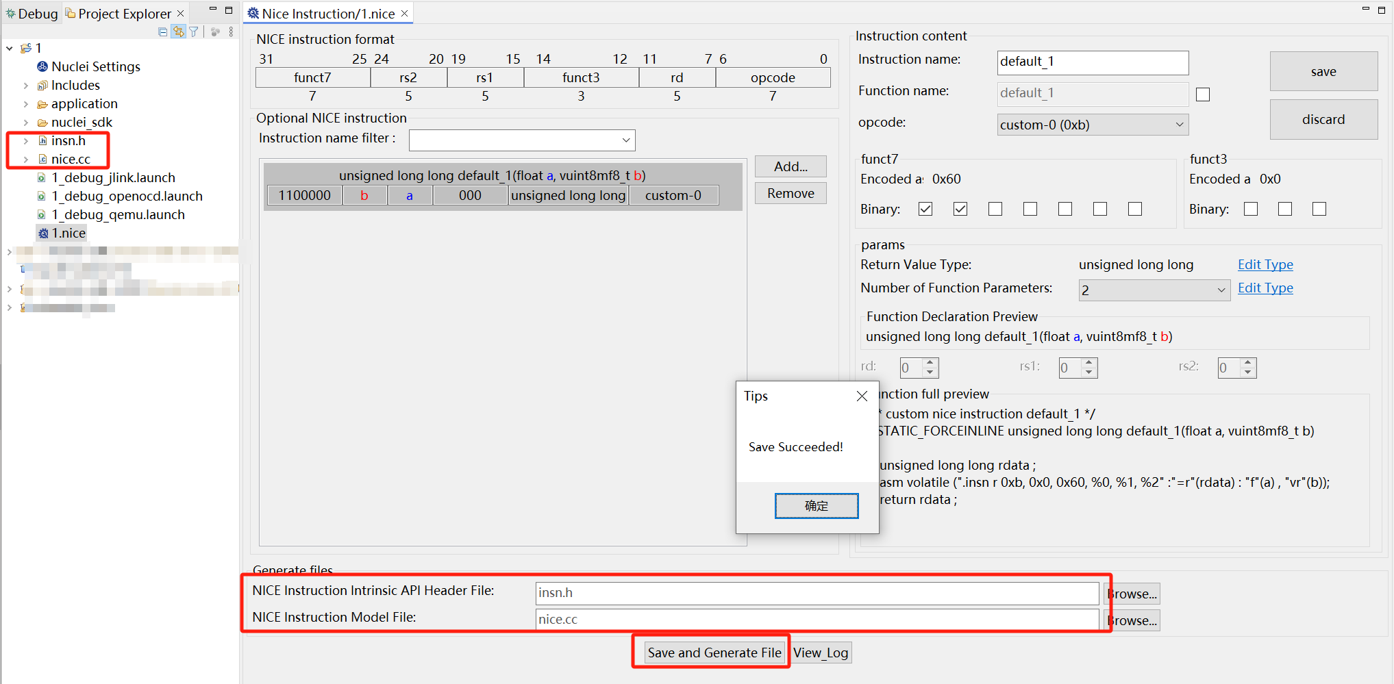
Define the save locations of the insn.h file (the inline assembly header) and the nice.cc file (the instruction implementation logic), then click Save and Generate File to generate the files.
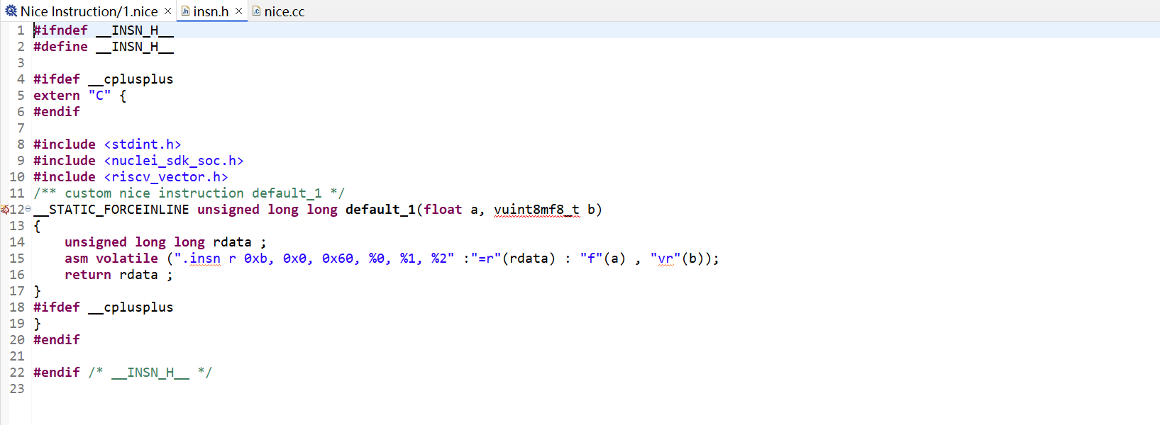
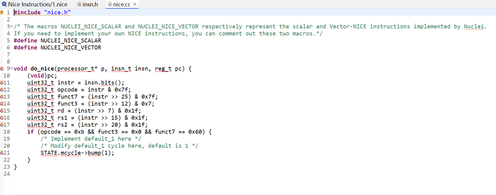
2.10.6.6. NICE Instruction Template Description
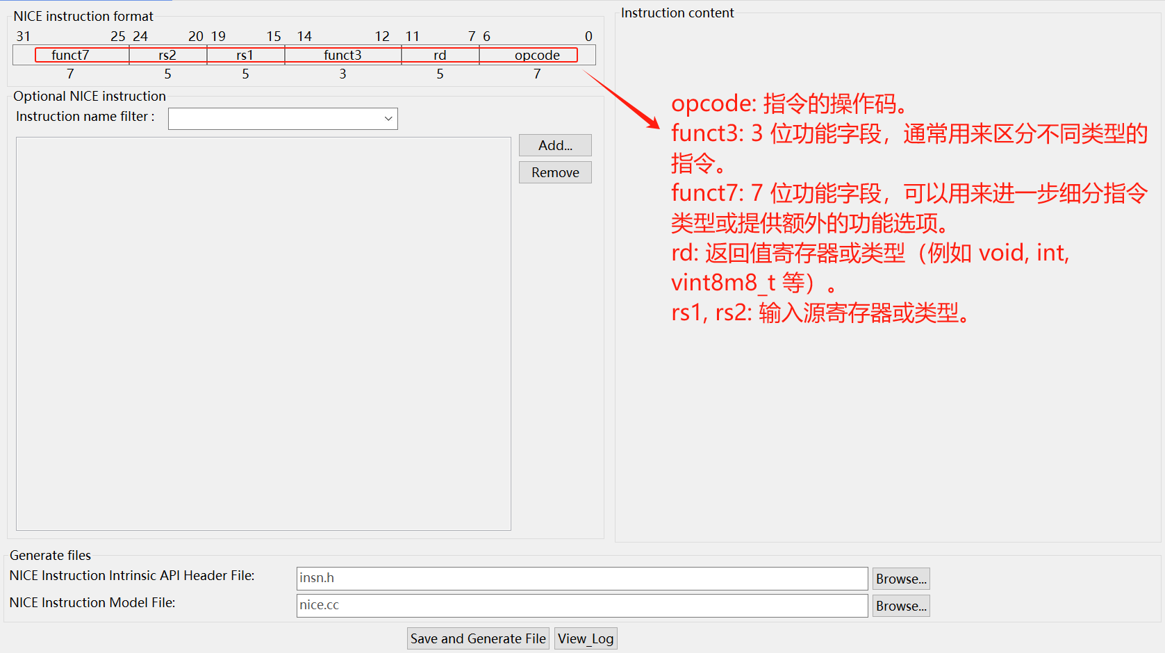
- A single instruction template is shown in the figure above:
opcode: custom-0, custom-1, custom-2, or custom-3
funct3: 3-bit function field, usually used to distinguish between different types of instructions.
funct7: 7-bit function field, which can be used to further subdivide instruction types or provide additional function options.
rd: return value register or type (for example void, int, vint8m8_t, etc.).
rs1, rs2: input source registers or types.
2.10.6.7. Instruction Content Editing Description
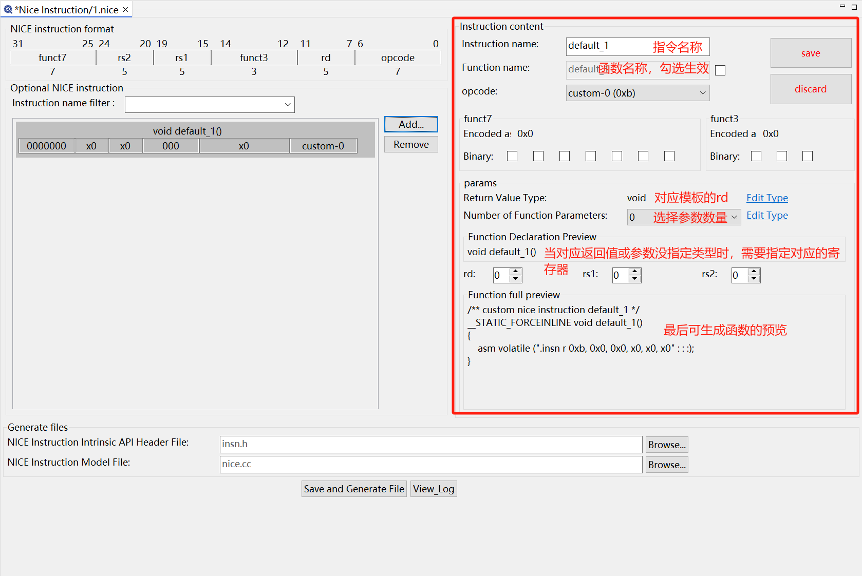
As shown above, the Instruction content area displays the default content.
Instruction name: the instruction name. The naming rules are as follows:
Letters and digits: the function name can contain letters
(A-Z, a-z)and digits(0-9), but cannot start with a digit.Underscore: underscores
_can be used in the function name to improve readability, especially in multi-word combinations. For example,get_user_nameis a valid function name;< , > , ... , ? , /are not allowed in a function name.Special characters: except for the underscore, other special characters such as
! , @ , # , $ , % , ^ , & , * , ( , ) , { , } , [ , ] , \ , : , ; ,are not allowed.Keywords: the function name cannot be a C language keyword or reserved word, such as
int , char , float , double , if , else , while , for , return.Function name: the function name. When not checked, the generated function name is the instruction name. The naming rules are the same as for
Instruction name.funct7: corresponds to the
funct7of the template, and can be set by checking the corresponding Binary items.funct3: corresponds to the
funct3of the template, and can be set by checking the corresponding Binary items.Return Value Type: corresponds to the rd of the template. Click Edit Type to set it, for example to void.
Number of Function Parameters: the number of parameters. You can set the types of the input parameters rs1, rs2, and rs3 (rs3 serves as both a parameter and a return value).
When the number of parameters is 0, Edit Type cannot be set. rs1 and rs2 can be assigned registers below; if rd is of void type, rd can also be assigned a register below.
When the number of parameters is 1, Edit Type can set the rs1 type. rs2 can be assigned a register below; if rd is of void type, rd can also be assigned a register below.
When the number of parameters is 2, Edit Type can set the rs1 and rs2 types. If rd is of void type, rd can also be assigned a register below.
When the number of parameters is 3, Edit Type can set the rs1, rs2, and rs3 types.
2.10.7. Using the Nuclei Model Debugger
Nuclei Model Debugger is a debugging and running tool developed for the upgraded Nuclei Near Cycle Model.
Starting with Nuclei Studio 2025.10, Nuclei Near Cycle Model provides richer features: it can debug and run programs and accepts custom parameters. To make these features easier to use, the Nuclei Model Debugger was developed based on the QEMU Debugger feature.
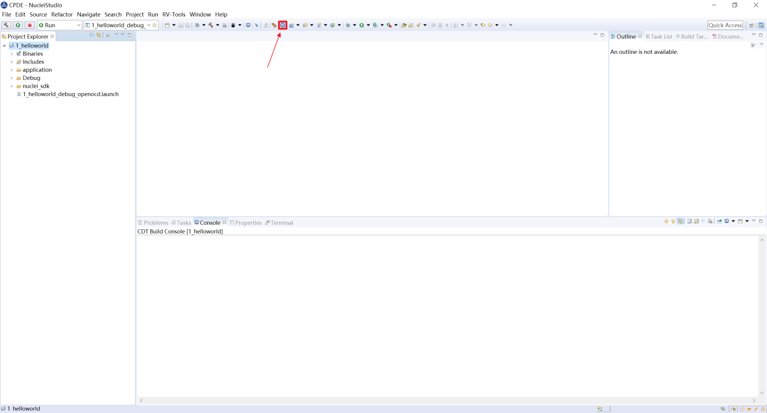
Create a test project and build it. In the Nuclei Studio main menu, click Run, then Run Configurations or Debug Configurations. This example uses Debug: click Debug Configurations.
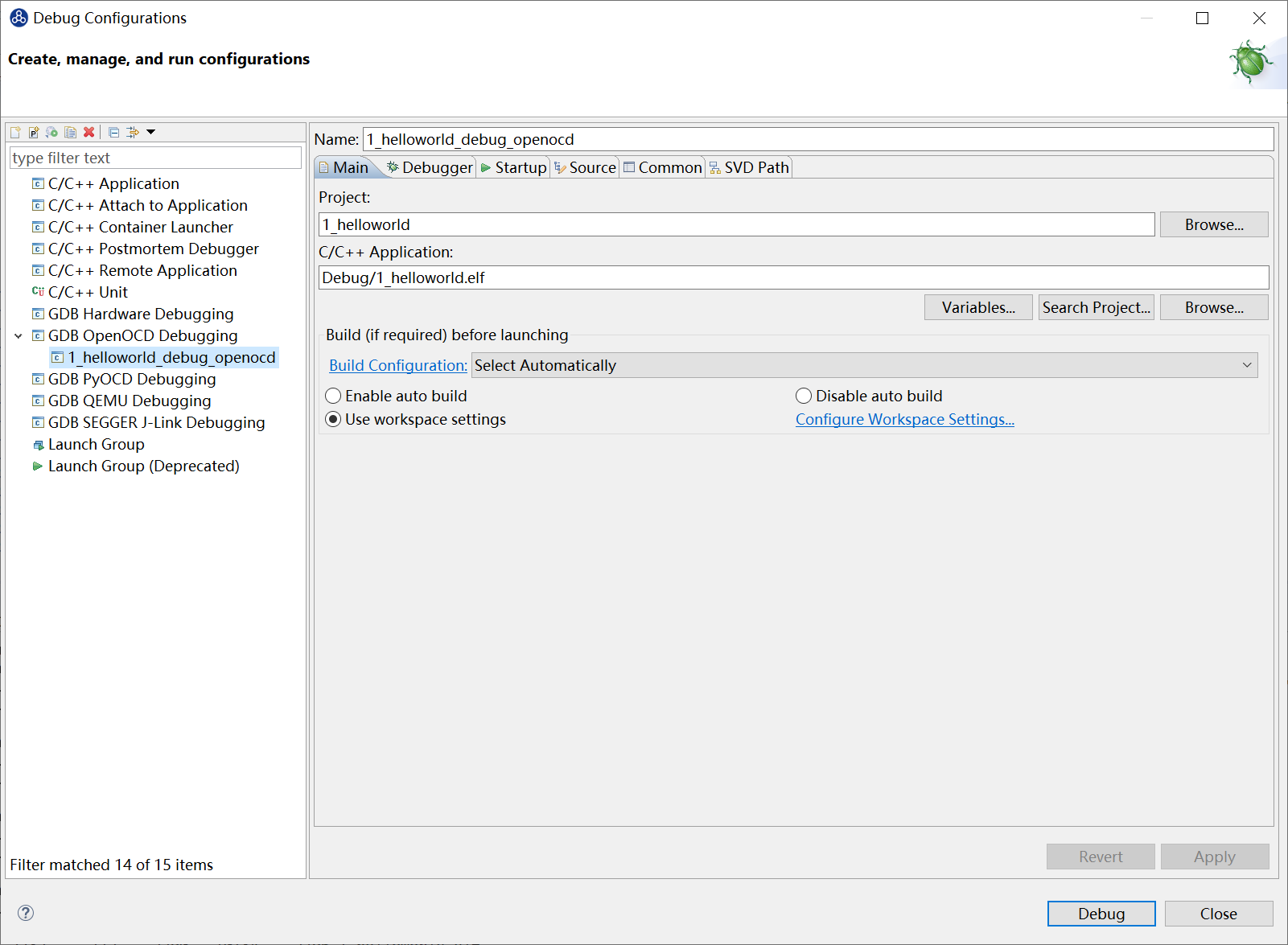
In the Debug Configurations dialog, find GDB Nuclei Model riscv Debugging.
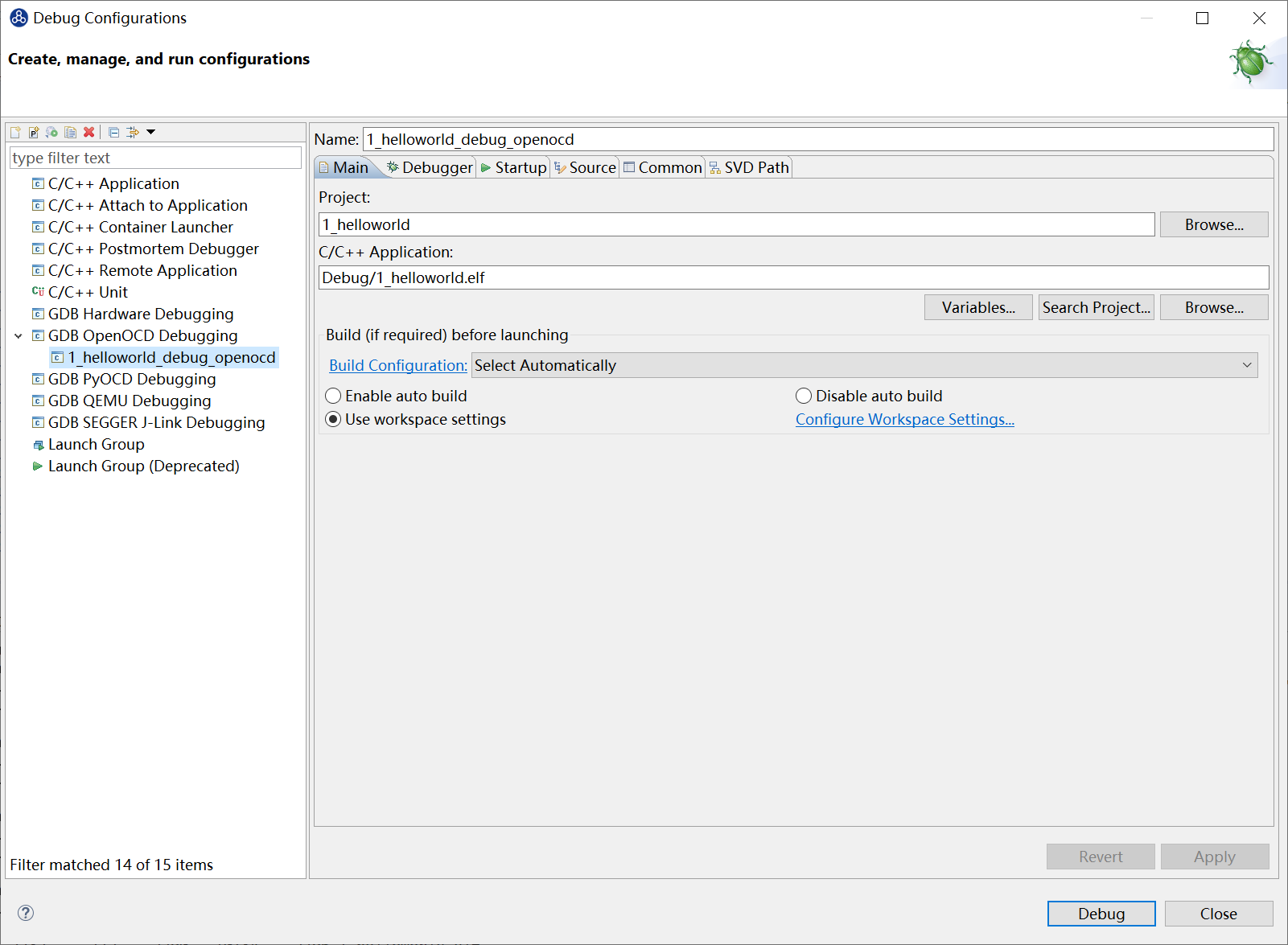
Double-click GDB Nuclei Model riscv Debugging, and Nuclei Studio creates a new Nuclei Model Debugger configuration page where you can configure the command parameters for Model Debug.

The values configured on the Debugger page must match the project.
Nuclei RISC-V Core The CPU core, which must match the program
Download Program download mode
Nuclei SMP Count CPU Number of cores
RVV length RISC-V vector extension
Other Extensions Other extensions
If Enable Nuclei Model RVTrace is checked and its path is configured, a *.rvtrace file is generated when the program runs.
In More options, you can add parameters supported by Nuclei Model. In this example, --gprof=1 --flame=1 is configured in Config options: --gprof=1 enables the gprof-based Profiling feature, so a gprof file is produced when the program runs, and --flame=1 enables the Flamegraph feature.
For details about the parameters of Nuclei Near Cycle Model, see Description of Parameters.
For the gprof Profiling feature, see Code Coverage and Profiling.
For the Flamegraph feature, see Using Flame View.
After configuring and saving the parameters, click Debug to enter the Nuclei Model Debug mode.
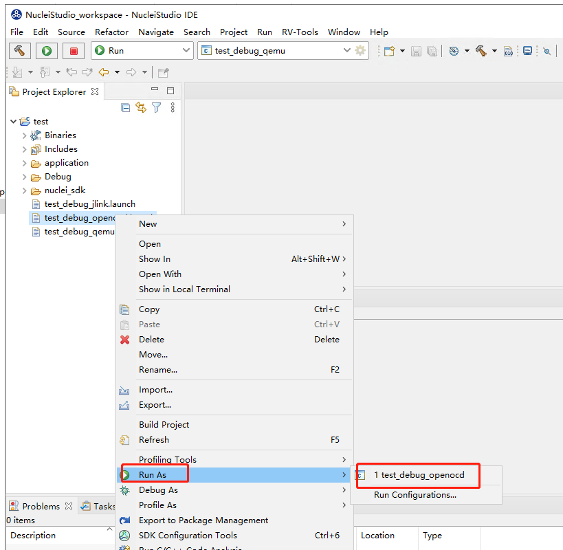
The program runs successfully in Nuclei Near Cycle Model and outputs the corresponding log information.

In the Debug directory of the project, you can see that the .rvtrace file and the .gmon file have been generated.

Nuclei Near Cycle Model supports analyzing programs with gprof. Therefore, when --gprof is configured, a .gmon file is also produced in the Debug directory (the directory configured with --logdir=XX) while the program runs. Double-click the .gmon file to invoke the gprof tool and analyze the number of cycles consumed by program execution and the call relationships; a corresponding callgraph.out file is also produced. Double-click the callgraph.out file to view the program’s call relationships with Call Graph.
The gprof tool displays the contents of the generated .gmon file.
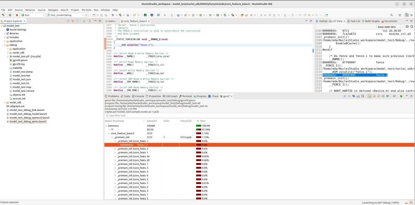
While viewing the .gmon file, the gprof tool parses the program’s call relationships based on its contents and generates a callgraph.out file. Double-click callgraph.out to view it with the Call Graph tool.
Because --flame=1 is configured, an xlmodel_flame_0.gtef file is produced in the project root directory. Double-click the file to invoke the Flame View tool to parse it and generate a flame graph.
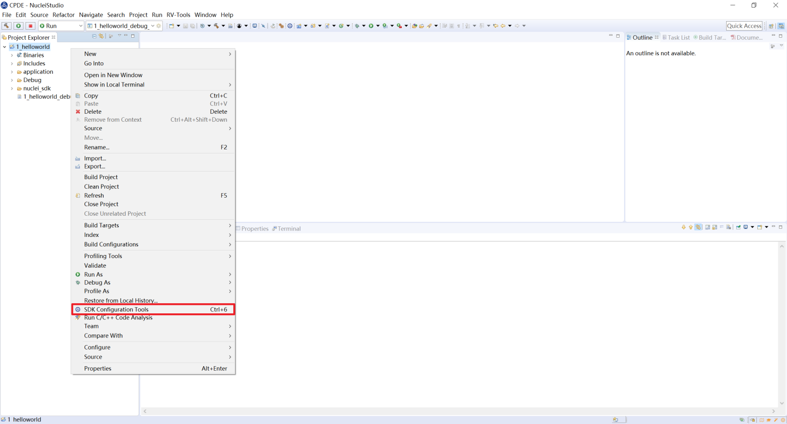
The same configuration supports both Debug and Run. To execute the program directly, switch in the Launch Bar.
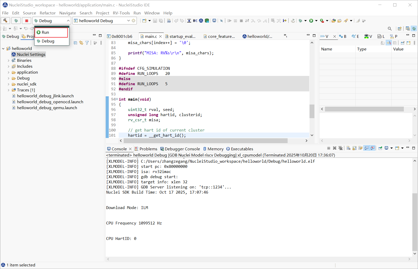
Click Run to enter Nuclei Model Run mode; the program executes directly to completion.

You can also export the configuration file to the project root directory so that it can be shared with other users.
Open the Debug Configurations page, right-click the configuration just created, and select `` Export… `` from the context menu.

In the Export Launch Configurations page, select the configuration to export and the export location, and click Finish to complete the export.
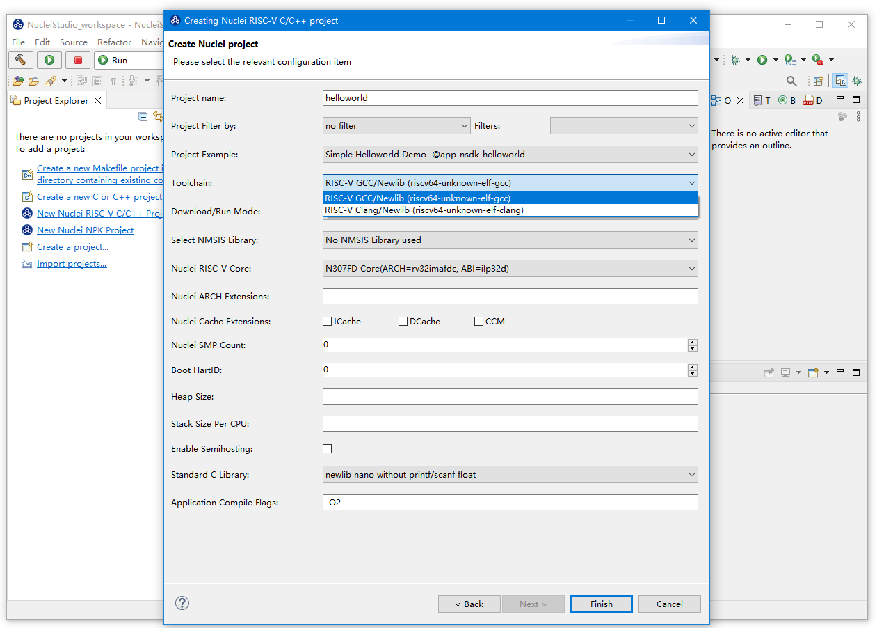
Refresh the project. A *.launch file exists under the project, and the corresponding configuration also appears in the Launch Bar. You can now use this configuration for Debug/Run operations on the program.
2.10.8. Using Nuclei Model
Nuclei has developed a dedicated running tool for Nuclei Near Cycle Model called Model. In Nuclei Studio 2024.06, Nuclei Near Cycle Model was originally run through the RVProf tool. As Nuclei Near Cycle Model continued to evolve, we simplified the RVProf-based functionality and launched the new Model tool to provide a simpler, more efficient user experience.
The main features of the new tool include:
Simplified functionality: removes unnecessary complex features so you can focus on the core functionality of Nuclei Near Cycle Model.
Improved efficiency: optimizes the operation flow and reduces configuration time.
Good compatibility: ensures seamless integration with existing workflows while supporting the latest Nuclei Near Cycle Model features.
With these improvements, you can use Nuclei Near Cycle Model for development and debugging more efficiently. Open Run Configuration via the Nuclei Studio menu Run -> Run Configuration, find Nuclei Model, and double-click it to generate the configuration for the project.

The use of Nuclei Model is described in detail in the Nuclei Near Cycle Model chapter.
2.10.9. Nuclei Near Cycle Model
Nuclei Studio 2024.06 integrates Nuclei Near Cycle Model, a simulation testing and performance analysis tool independently developed by Nuclei. It helps R&D personnel perform simulation testing and program performance analysis in the early stages of a project.
Nuclei Near Cycle Model is only available for Linux in Nuclei Studio 2024.06; Windows support was added in version 2025.02. For a detailed introduction and command line usage, see https://doc.nucleisys.com/nuclei_tools/xlmodel/intro.html. The following sections demonstrate how to use Nuclei Near Cycle Model for simulation and performance analysis in Nuclei Studio.
Note
Nuclei Near Cycle Model now supports both Windows and Linux. The tests in this document were all performed with the Windows version of Nuclei Studio IDE 2025.02.
If you encounter any problems during use, check https://github.com/Nuclei-Software/nuclei-studio or submit an issue.
2.10.9.1. Creating a Test Project
Nuclei Near Cycle Model supports all types of Nuclei cores. Create any demo project and build it.

Nuclei Near Cycle Model runs tests using the Model run configuration in Nuclei Studio. Select the built test project, and then open Run Configurations in Nuclei Studio.

Create a Nuclei Near Cycle Model configuration. The configuration parameters are described below.

In this example, --trace=1 --gprof=1 --logdir=Debug --cpu=n300fd is configured in Config options: --trace=1 enables rvtrace, --gprof=1 enables the gprof feature, --logdir=Debug stores the generated .rvtrace and .gmon files in the Debug directory under the current project, and --cpu=n300fd sets the simulated CPU core to n300fd.
Note
--cpu=<core type> must be configured and must be consistent with the Core value configured in Nuclei Setting.
--ext=<extension type> must be consistent with the Other extensions value configured in Nuclei Setting.
For details about the parameters of Nuclei Near Cycle Model, see Description of Parameters.
2.10.9.2. Running the Project and Generating Profiling Results
Click the Run button to run the program. The program runs successfully in Nuclei Near Cycle Model and outputs the corresponding log information.
In the Debug directory of the project, you can see that the .rvtrace file and the .gmon file have been generated.
Nuclei Near Cycle Model supports analyzing programs with gprof. Therefore, when --gprof is configured, a .gmon file is also produced in the Debug directory (the directory configured with --logdir=XX) while the program runs. Double-click the .gmon file to invoke the gprof tool and analyze the number of cycles consumed by program execution and the call relationships; a corresponding callgraph.out file is also produced. Double-click the callgraph.out file to view the program’s call relationships with Call Graph.
The gprof tool displays the contents of the generated .gmon file.
While viewing the .gmon file, the gprof tool parses the program’s call relationships based on its contents and generates a callgraph.out file. Double-click callgraph.out to view it with the Call Graph tool.
2.10.10. Using the GDB Custom Debugging Feature
GDB Custom is a simplified debug configuration developed by Nuclei to accommodate different debugging tools. It lets you debug programs in Nuclei Studio with your own custom debugging tools. GDB Custom supports debugging projects through Commands, Generic Serial, and DLink; choose the method that fits your setup.
The GDB Custom debugging feature is illustrated with DLink, a debugging tool developed by Nuclei. For details, see Debugging and Running a Project with DLink.
2.10.11. Using Live Watch
Live Watch is a real-time monitoring tool that helps you debug and optimize code more efficiently. With Live Watch, you can view variable changes instantly while the program is running, without interrupting execution or adding log statements manually. Live Watch was introduced in Nuclei Studio 2025.02. It refreshes variable values automatically so that you always see the latest data, and its intuitive graphical interface makes it easy to manage the variables you want to monitor.
Note
The Live Watch feature depends on Nuclei OpenOCD >= 2025.02. It is only supported on Nuclei CPUs configured with the RISC-V SBA feature.
2.10.11.1. Live Watch Overview
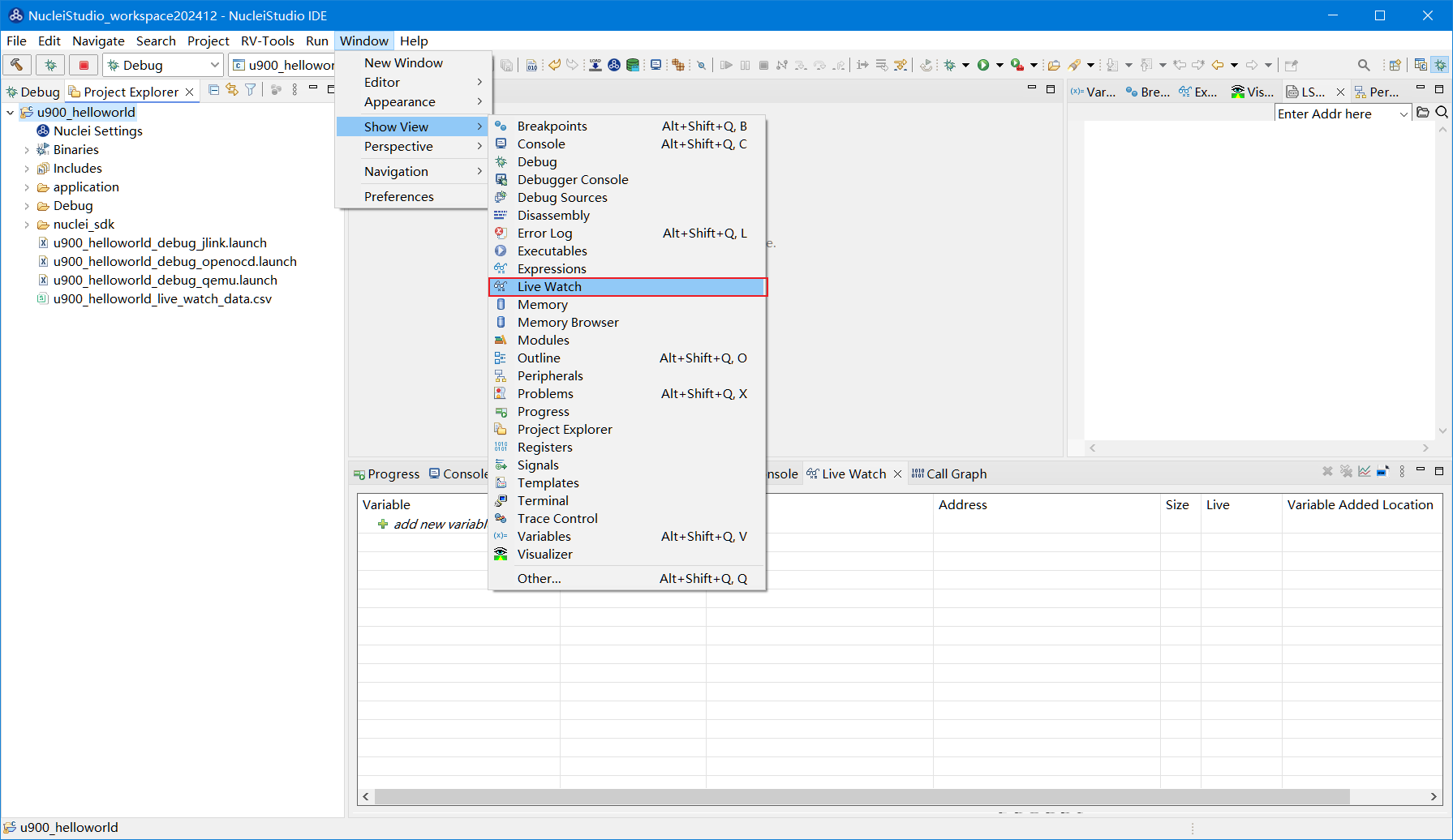
Open the Live Watch view via the Nuclei Studio menu Window -> Show View -> Live Watch.
The Live Watch view provides several function menus to help you manage and monitor variables:
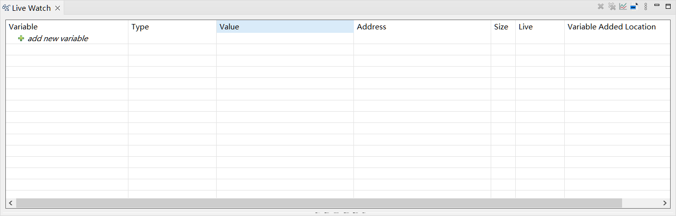
Remove
Deletes the selected variable row from the Live Watch view.
Remove All
Clears all variables added to the Live Watch view.
Show Live Plot
Shows the Live Plot view, which plots the sampled data in real time.
The hidden menu bar contains two settings menus for configuring global properties:
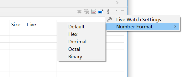
Live Watch Settings
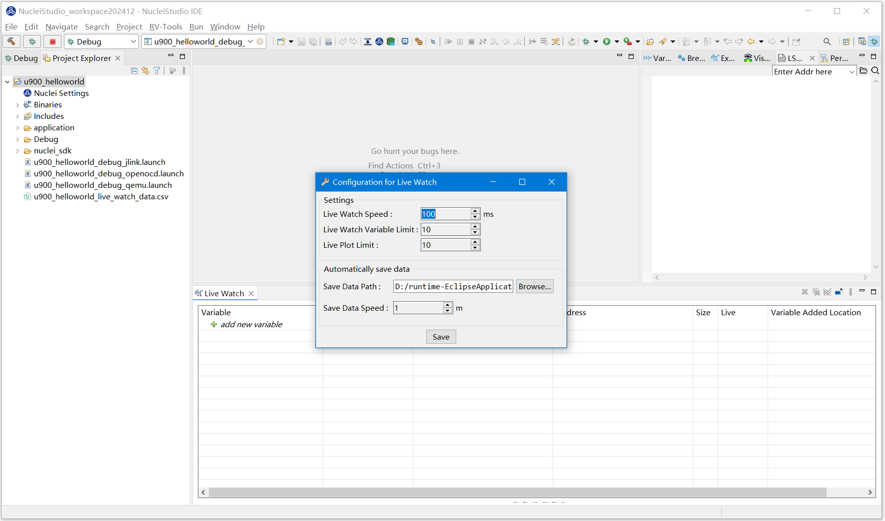
Common settings in Live Watch:
The following settings are available:
Live Watch Speed : sets the sampling frequency of Live Watch, up to once every 1 ms. A sampling period of 5 ms or longer is recommended; if the sampling frequency is too high, Live Plot may draw abnormally.
Live Watch Variable Limit : limits the number of variables sampled at the same time, up to 10.
Live Plot Limit : sets the maximum number of samples that Live Plot draws at the same time, up to 10.
Save Data Path : specifies the path where the data sampled by Live Watch is automatically saved, for subsequent analysis.
Save Data Speed : sets the frequency at which Live Watch data is automatically saved. The default is once every 10 minutes.
Number Format
Sets the display format of variable values in the Live Watch view.
2.10.11.2. Live Watch Demo
Create a test project and implement a sine calculation in it. Open the Live Watch view, find Live Watch Settings, and set the related parameters as needed (or keep the default values).

#include <stdio.h>
#include "nuclei_sdk_soc.h"
#include <math.h>

#define PI 3.14159265358979323846
/**
* Get a sine wave variable that varies with time
*/
double get_sine_wave_value(double amplitude, double frequency) {
   // Get the value of the current cycle counter
   uint64_t current_cycle = __get_rv_cycle();

   // Calculate the current time (in seconds)
   double currentTime = (double)current_cycle / SystemCoreClock;

   // Precompute the frequency-related factor
   double omega = frequency * 2 * PI;

   // Calculate the phase
   double phase = currentTime * omega;

   // Return the sine value
   return sin(phase) * amplitude;
}

int main(void)
{

   double amplitude = 100.0; // amplitude of the waveform

   double frequency = 0.1;  // frequency of the waveform (cycles per second)

   double sine_value = 0;

   printf("Enter to task_2\r\n");
   while (1) {

      sine_value = get_sine_wave_value(amplitude, frequency);

   }

   return 0;
}
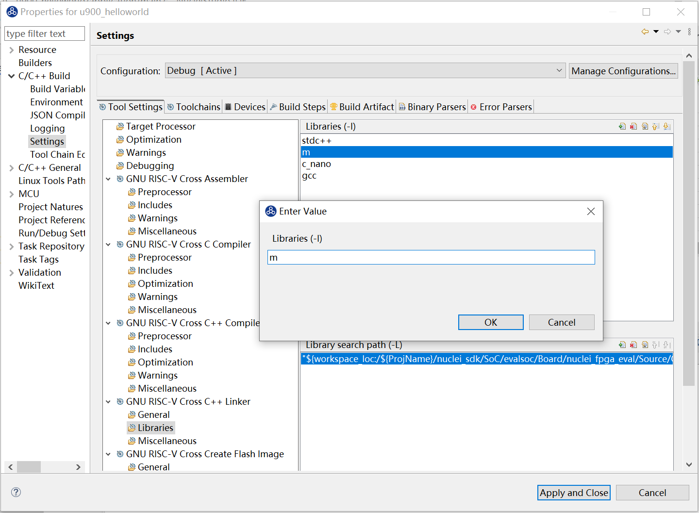
The test demo uses math functions, so you need to add -lm to the linker options. In the project properties, go to Settings -> GNU RISC-V Cross C++ Linker -> Libraries and add -lm.
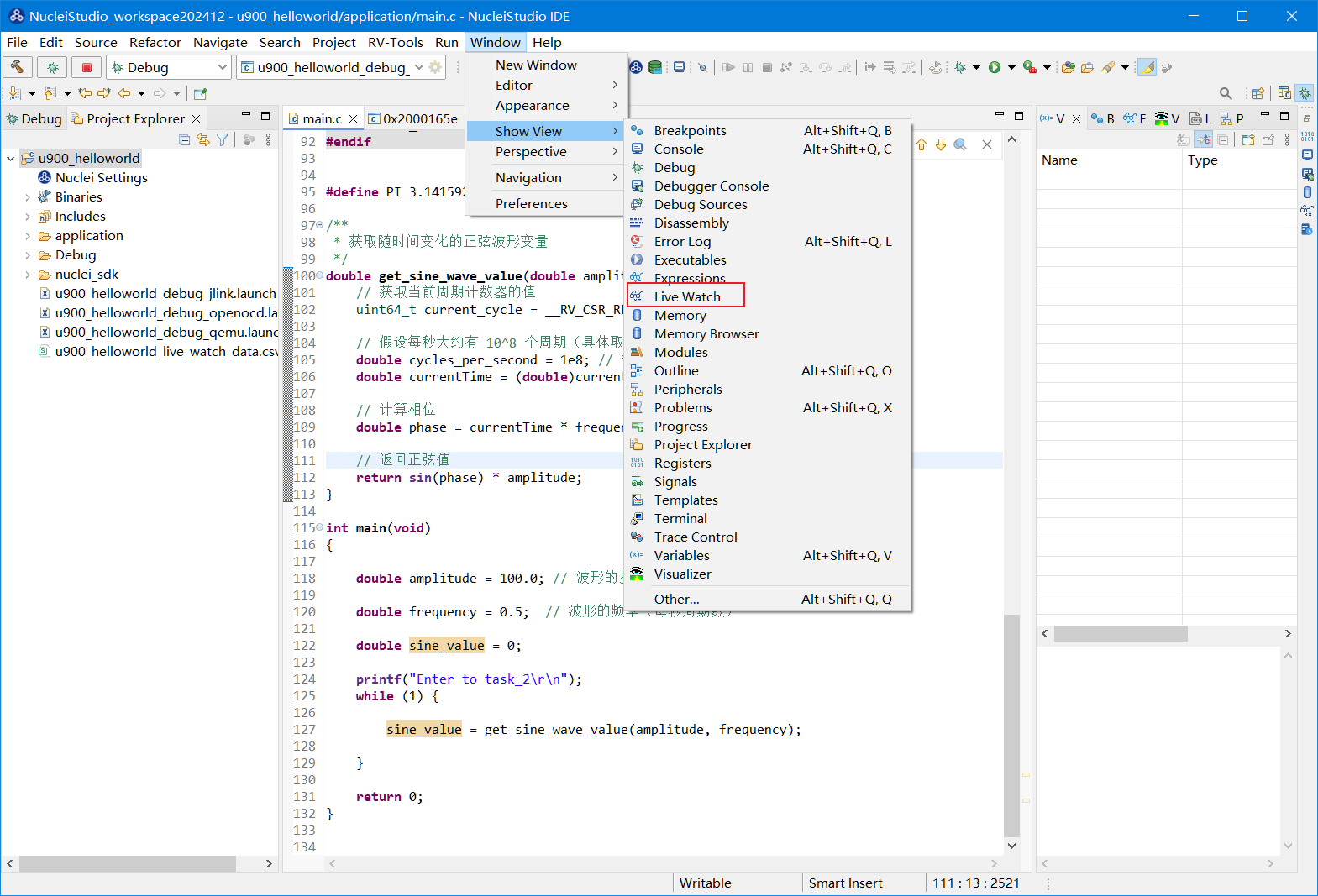
Open the Live Watch view via Windows -> Show View -> Live Watch.
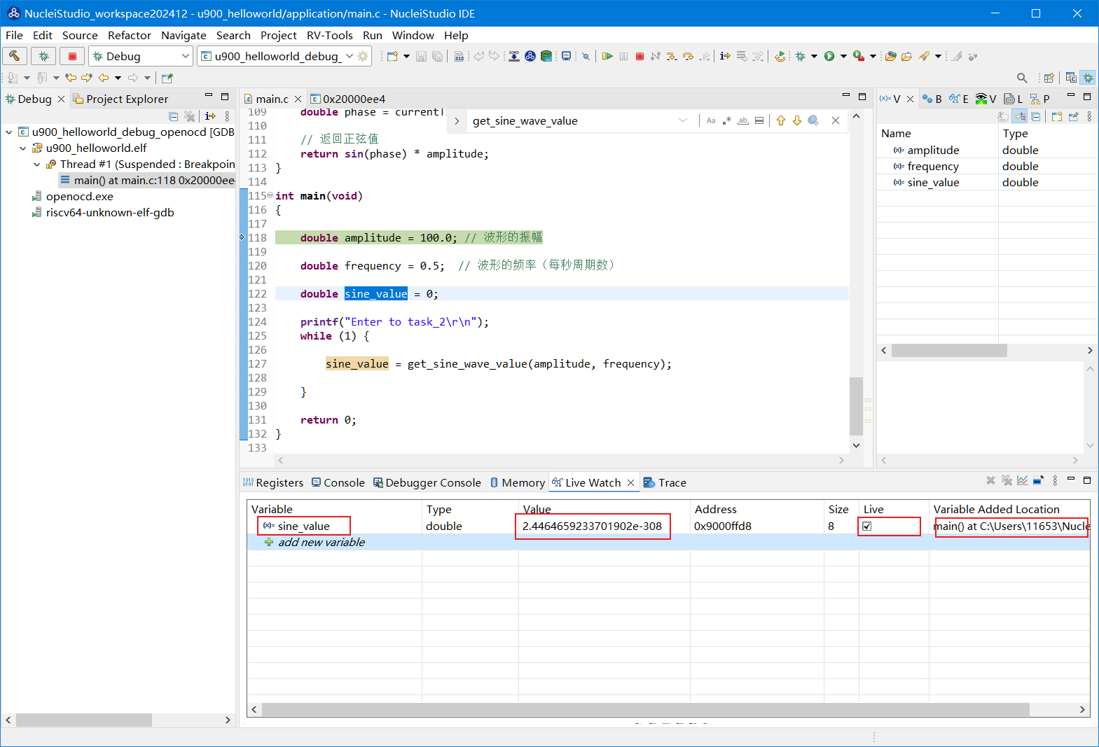
After building the project and running the program in Debug mode, add the variables you want to view in the Live Watch view. There are two ways to add variables: click add new variable in the Live Watch window to add them manually, or select a variable in the project and drag it into the Live Watch window with the left mouse button.
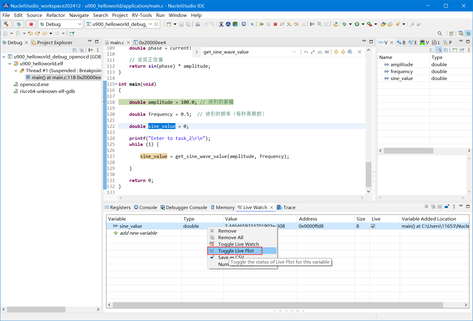
When the program runs at full speed, the variable values change at the configured Live Watch Speed. To view a variable’s change curve with Live Plot, select the record, right-click, and select Toggle Live Plot from the context menu. The Live Plot tool opens and draws the variable’s change curve.
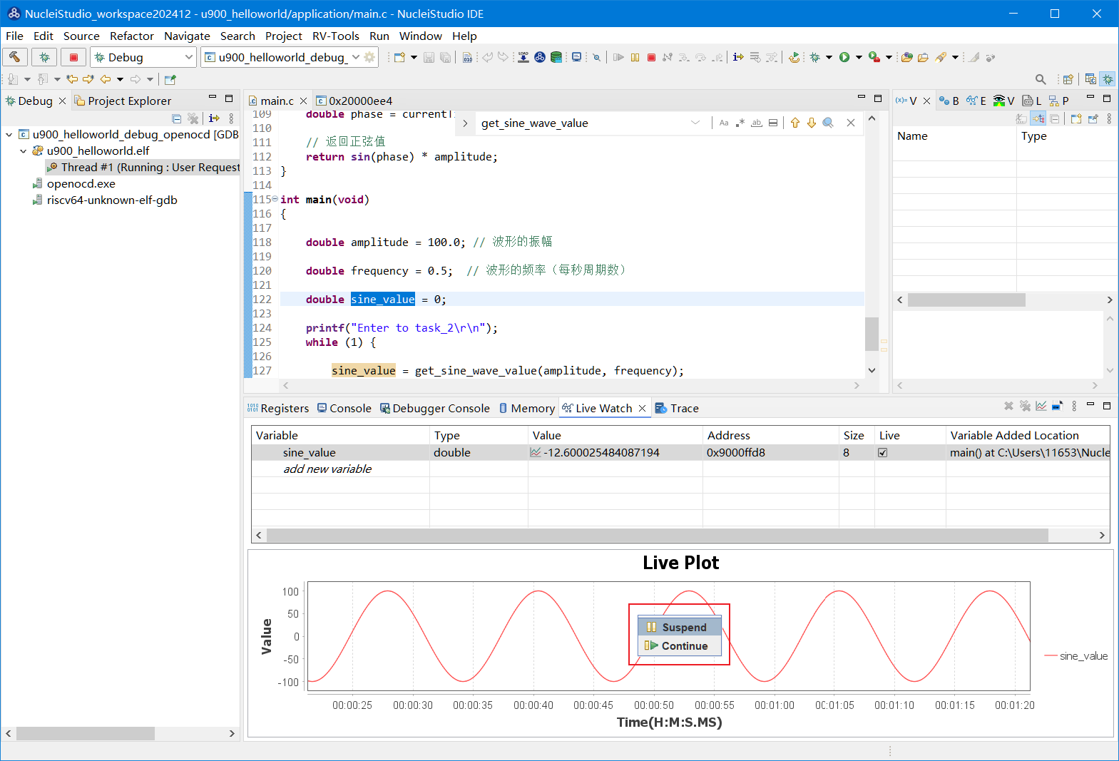
The curve drawn by Live Plot is shown below.

Right-click in Live Plot to open a menu with two items, Suspend and Continue. Click Suspend to pause drawing.
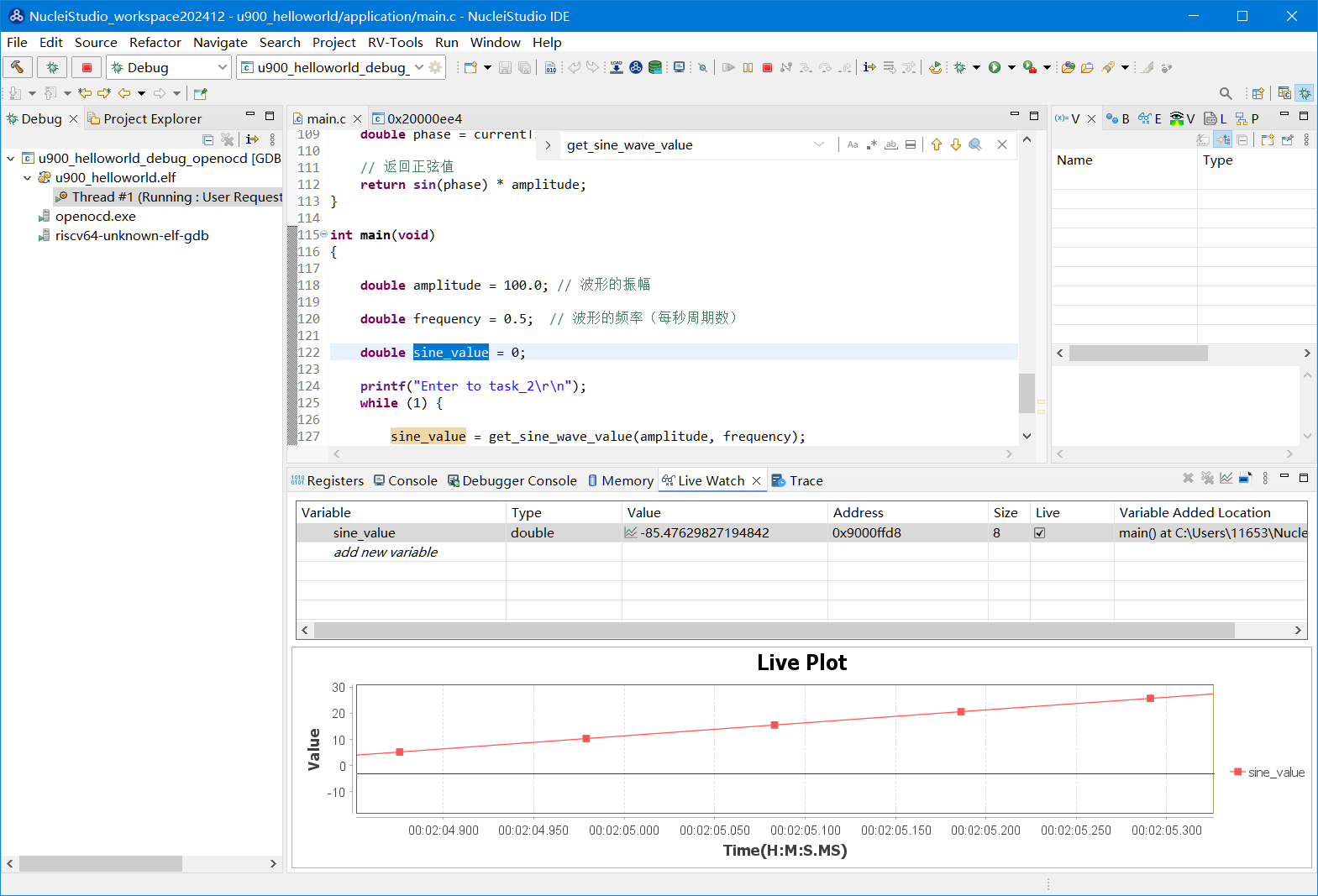
Scroll the mouse wheel to zoom in on the curve and view data details; click Continue to resume drawing.
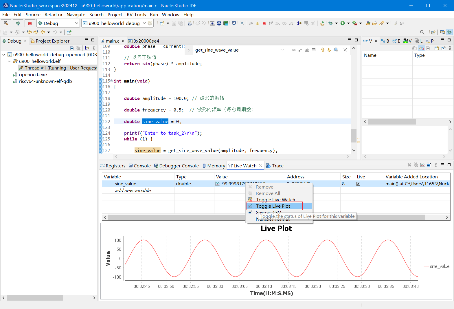
If you no longer want to view the change curve of a variable, click Toggle Live Plot again to remove the variable from Live Plot.
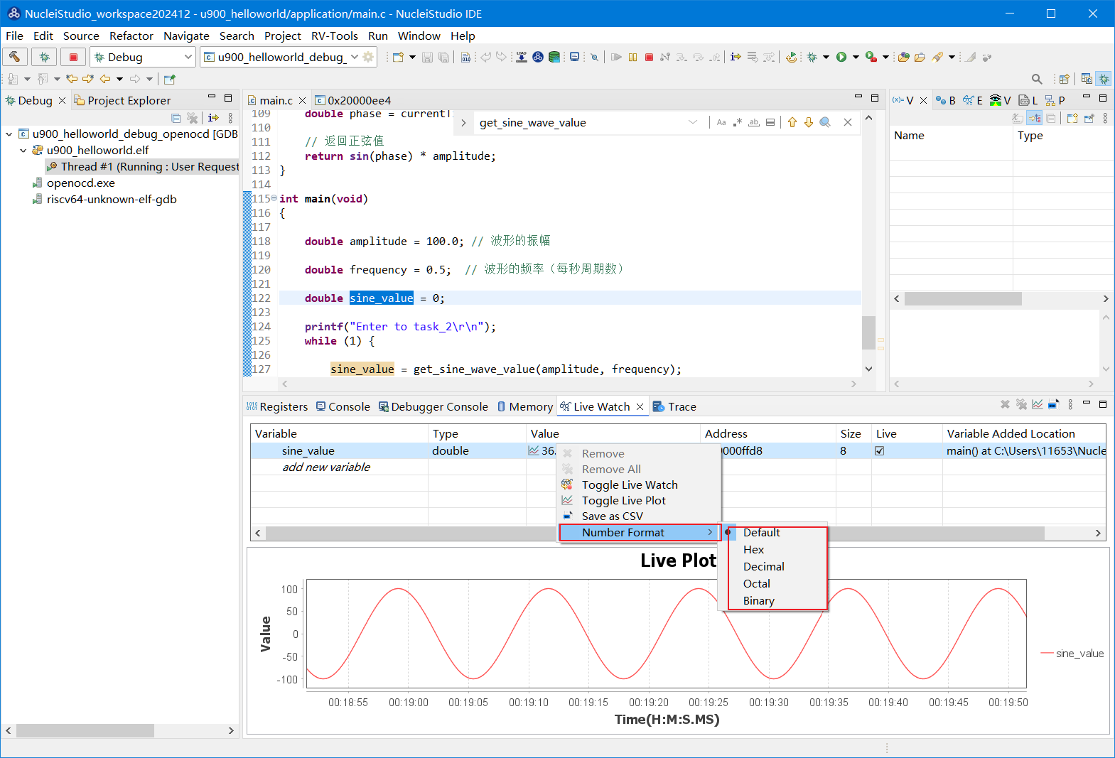
Right-click a variable in the Live Watch view to modify the display format of its data.
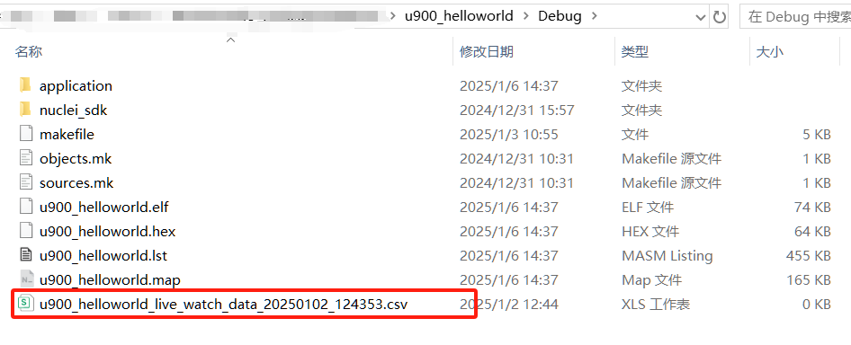
Right-click a variable in the Live Watch view to save its sampled results as a CSV file for later use.

Live Watch also automatically saves the sampled data to Save Data Path, where you can find the corresponding CSV files.
To stop watching a variable, select the record, right-click, and select Toggle Live Watch from the context menu. Live Watch then stops querying the variable’s value in real time.

2.10.11.3. Troubleshooting Live Watch
Dependency on RISC-V SBA
As mentioned earlier, Live Watch depends on RISC-V SBA. If Live Watch cannot obtain a variable’s value, the current CPU may not support RISC-V SBA. Use the following method to confirm whether the CPU supports RISC-V SBA.
While the project is in the Debug state, obtain the address of the variable in Live Watch, as shown below.
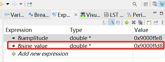
Open the telnet tool, configure it, and connect. If the connection fails, check whether the OpenOCD service has started properly and whether the telnet port is open.

While still in the Debug state, use the command riscv set_mem_access sysbus in the telnet tool to set the riscv memory access mode to sysbus (SBA), and try to read the value of the variable.
> riscv set_mem_access sysbus
> mdw 0x9000ffd8 4
0x9000ffd8: 000ab156 404e8df0 9999999a 3fb99999
If the operation above reads the variable’s value, run the program at full speed and read the value again. If no error is reported and the value can be read, the current CPU supports the SBA feature.
> mdw 0x9000ffd8 4
0x9000ffd8: 000ab156 404e8df0 9999999a 3fb99999
> mdw 0x9000ffd8 4
0x9000ffd8: d0b53424 c0510557 9999999a 3fb99999
> mdw 0x8000ffd8 4
0x8000ffd8: 00000000 00000000 00000000 00000000
> mdw 0x9000ffd8 4
0x9000ffd8: b169d356 c0580176 9999999a 3fb99999
> mdw 0x9000ffd8 4
0x9000ffd8: a69861c1 c056547d 9999999a 3fb99999
> mdw 0x9000ffd8 4
0x9000ffd8: 4dbf49f2 404022d3 9999999a 3fb99999
> mdw 0x9000ffd8 4
Live Watch Cannot Read Variable Values When the Optimization Level Is Too High
When the project’s optimization level is high, Live Watch may not be able to obtain the values of some variables, as demonstrated below.
int test()
{
   uint32_t live_watch = 0;
   while(1){
      live_watch += 1;
      delay_ms(100U);
   }
}
When the project’s optimization level is set to O3 or higher, Live Watch cannot obtain the value of live_watch. You can lower the project’s optimization level, or declare the monitored variable as a global or static variable so that it is not optimized away by the compiler. Modify the project code as follows.
int test()
{
   static uint32_t live_watch = 0;
   while(1){
      live_watch += 1;
      delay_ms(100U);
   }
}
2.10.12. Using Flame View
Flame View is an intuitive and efficient performance analysis tool for visualizing the execution call stack and time distribution of programs in embedded systems. By converting complex trace data into a hierarchical stacked graph, Flame View helps developers quickly identify hot functions, analyze execution paths, and locate performance bottlenecks.
The *.gtef file is a file format defined in the IDE specifically for the Flame View tool. Currently, a *.gtef file can be parsed from Trace data (see Using Flame View with Trace) or produced directly by Nuclei Model (see Using Flame View in Nuclei Model).
If you already have a *.gtef file, simply double-click the file to start the Flame View tool. A guide prompt pops up first, informing you that the IDE will import the *.gtef file into the Traces directory.
At the same time, the IDE opens the Flame Chart view and the Flame Graph view.

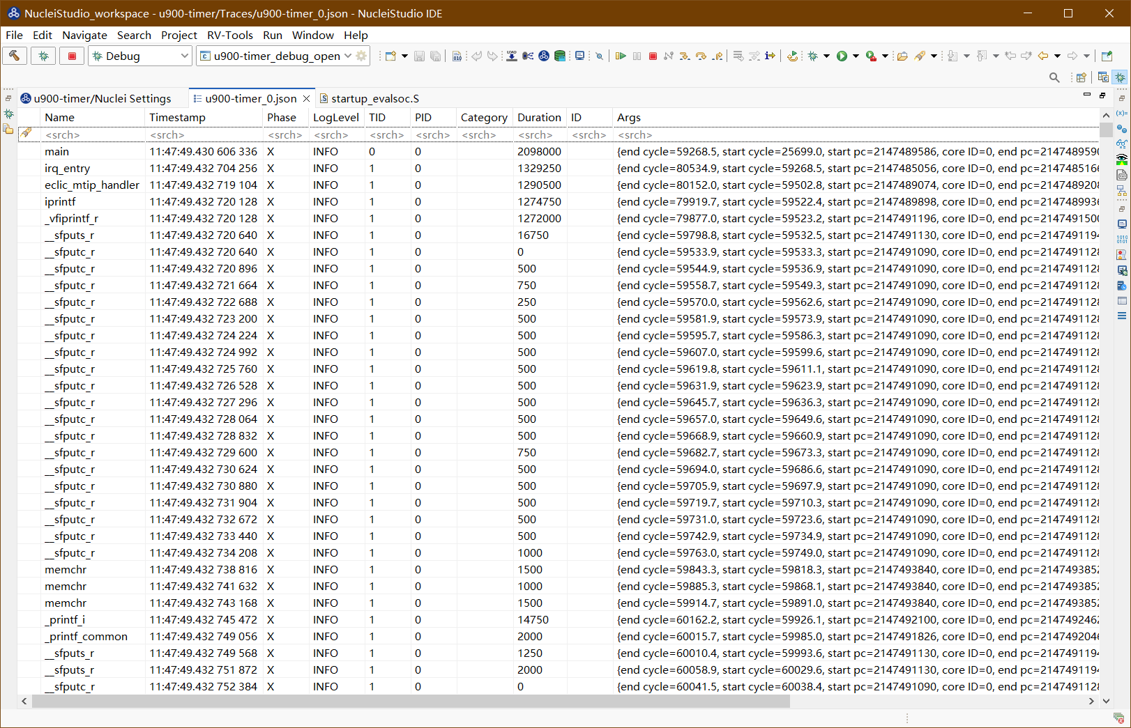
The Flame Chart view shows function-related information in list form, such as start time and execution duration.
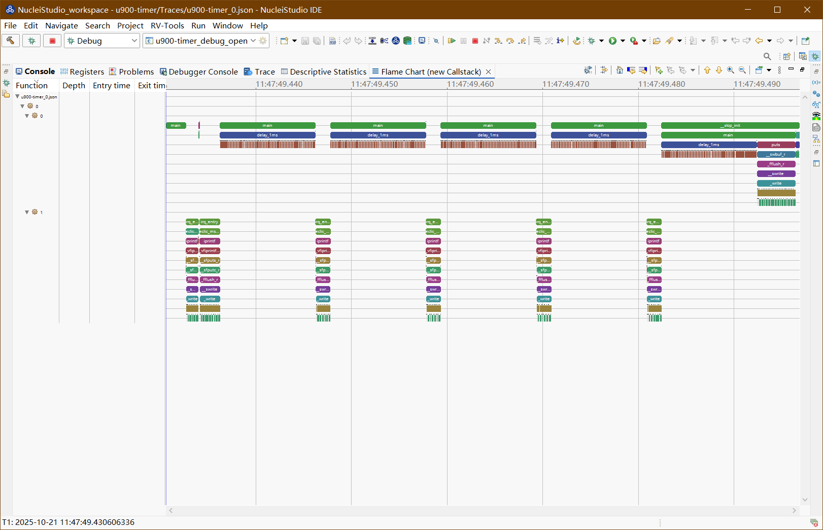
The Flame Graph view shows the execution time, call hierarchy, execution duration, and other data of each function as a flame graph. In the Flame Graph view, use A D W S to zoom in and out and view more detailed information.
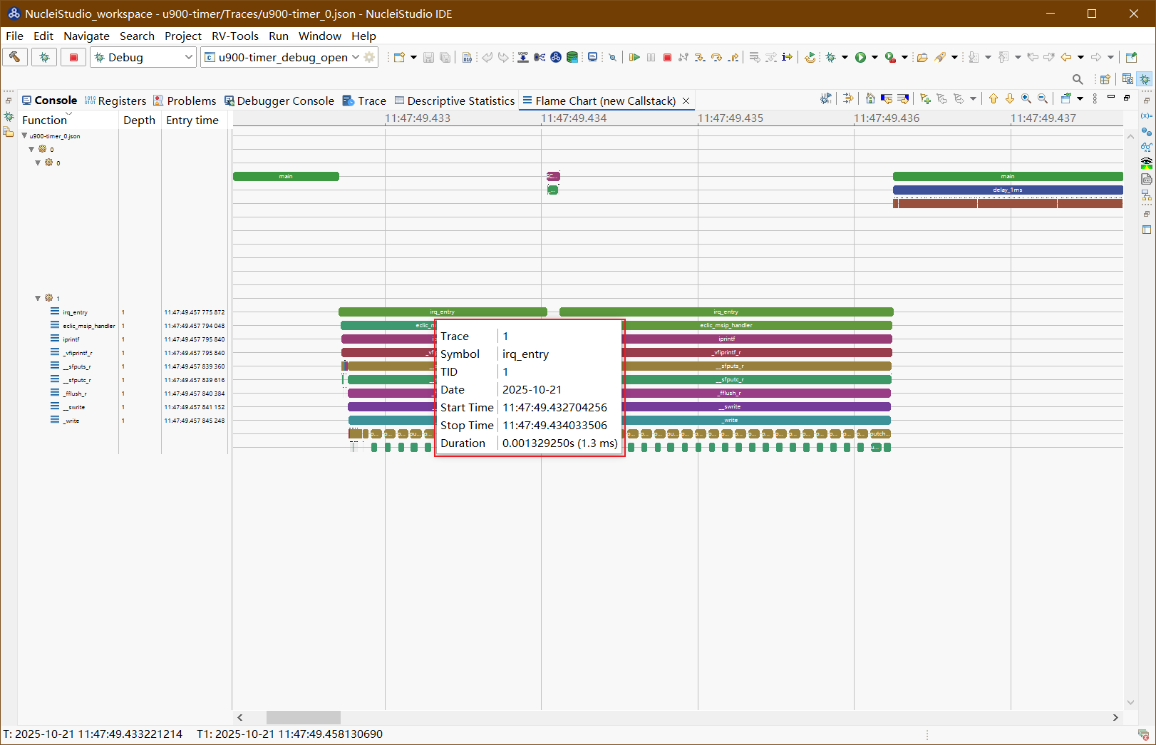
Click a segment in the flame graph to display more detailed information about it.
With the flame graph, you can understand the execution and time consumption of the program, quickly identify hot functions, analyze execution paths, and locate performance bottlenecks.
The *.gtef file can also be displayed with Google’s open-source Perfetto Trace Viewer. Open https://ui.perfetto.dev/, click Open trace file, find the *.gtef file generated in the project, and load it into Perfetto.
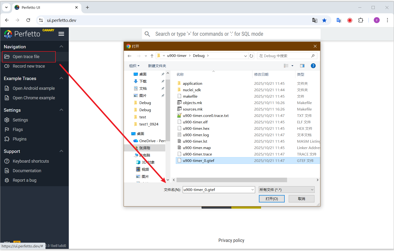
In the flame graph, use A D W S to zoom in and out and view more detailed information.

2.10.13. Flash Programming
Nuclei Studio provides the Flash Programming feature for downloading compiled binary files directly to hardware development boards quickly and conveniently, greatly improving development and debugging efficiency. The operation flow is simple: after the project is built, click Flash Programming to download the binary file in one step.
For details, see Flash Programming.
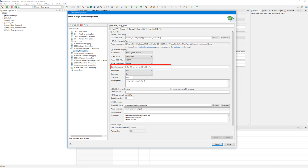
2.10.14. Connect to Running Target
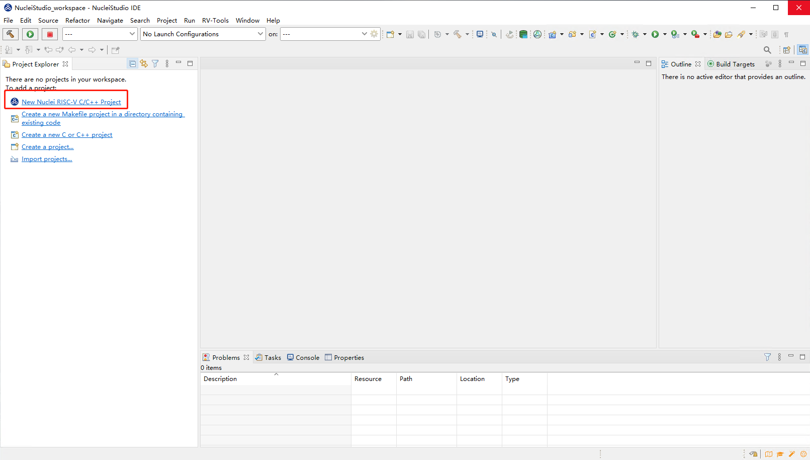
Nuclei Studio provides the Connect to Running Target feature for connecting directly to a running development board. It connects to the running board and reads board information, greatly improving development efficiency.
For details, see Connect to Running Target.
2.10.15. Updating evalsoc Configuration in Nuclei QEMU
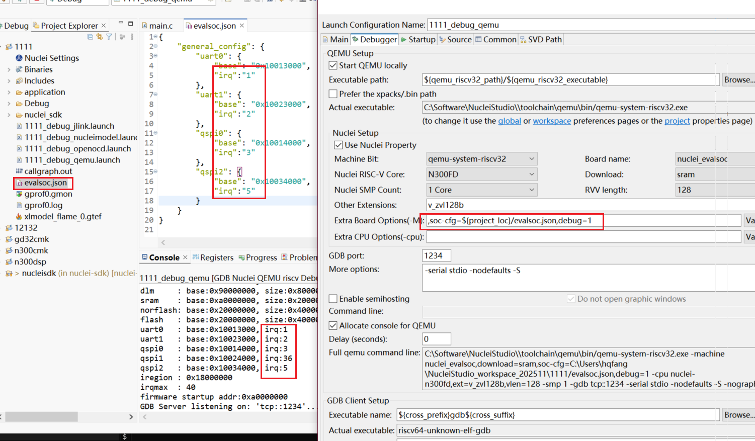
To let you quickly modify the addresses and sizes of peripherals and the interrupt numbers in the Nuclei QEMU evalsoc — without modifying the Nuclei QEMU source code — and thus adapt to different evalsoc versions, Nuclei QEMU extends the -M option with the soc-cfg option. You write a json configuration file and pass an option such as -M nuclei_evalsoc,download=ddr,soc-cfg=evalsoc.json,debug=1 on the QEMU command line to modify the evalsoc peripheral configuration.
In Nuclei Studio, place the evalsoc.json file in the root directory of your project, then modify Extra Board Options(-M) on the Debugger Tab of the Nuclei QEMU Debug Configuration page. Change it to ,soc-cfg=${project_loc}/evalsoc.json,debug=1 and save the debug configuration.
You can then debug Nuclei QEMU features according to the new evalsoc configuration.
2.10.16. Switching From the GNU GCC Toolchain to the Clang/ZCC Toolchain
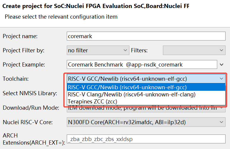
Nuclei Studio IDE supports three toolchains: RISC-V GCC/Newlib, RISC-V Clang/Newlib, and Terapines ZCC.
When creating a project, select the desired toolchain in the Toolchain drop-down box.
If the current project uses the GCC toolchain and you want to switch to the Clang or ZCC toolchain, you can complete the migration with the following steps:
2.10.16.1. Switching the Toolchain
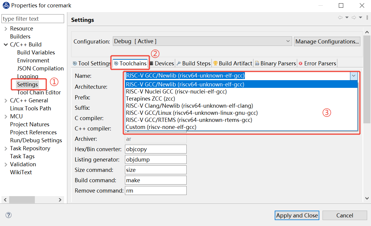
Select the project in Project Explorer, right-click and select Properties to open the project properties, then go to C/C++ Build -> Settings -> Toolchains and select the target toolchain in the Name drop-down box.
2.10.16.2. Adjusting Compile and Link Options
2.10.16.2.1. RISC-V Clang/Newlib
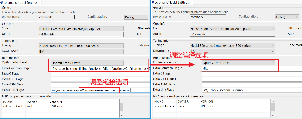
If you switch to the Clang toolchain, you need to adjust the compile and link options accordingly, because Clang is not fully compatible with all GCC parameters.
Taking the CoreMark project as an example, the parameters used by different CPU series may vary slightly, but the following adjustments are generally recommended:
Change
Optimization Levelfrom-Ofastto-O3;Replace
Extra Common Flagswith-flto;Remove
-Wl,--no-warn-rwx-segmentsfrom the link options.
2.10.16.2.2. Terapines ZCC
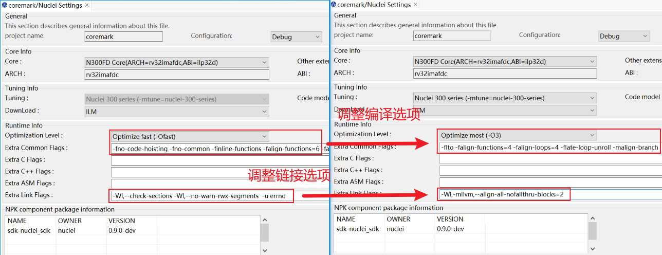
If you switch to the ZCC toolchain, it is recommended to adjust the compile and link options as follows:
Change
Optimization Levelfrom-Ofastto-O3;Replace
Extra Common Flagswith-flto -falign-functions=4 -falign-loops=4 -flate-loop-unroll -malign-branch;Remove
-Wl,--no-warn-rwx-segmentsfrom the link options;Change the link options to
-Wl,-mllvm,--align-all-nofallthru-blocks=2.
2.10.16.3. Adjusting Linked Libraries
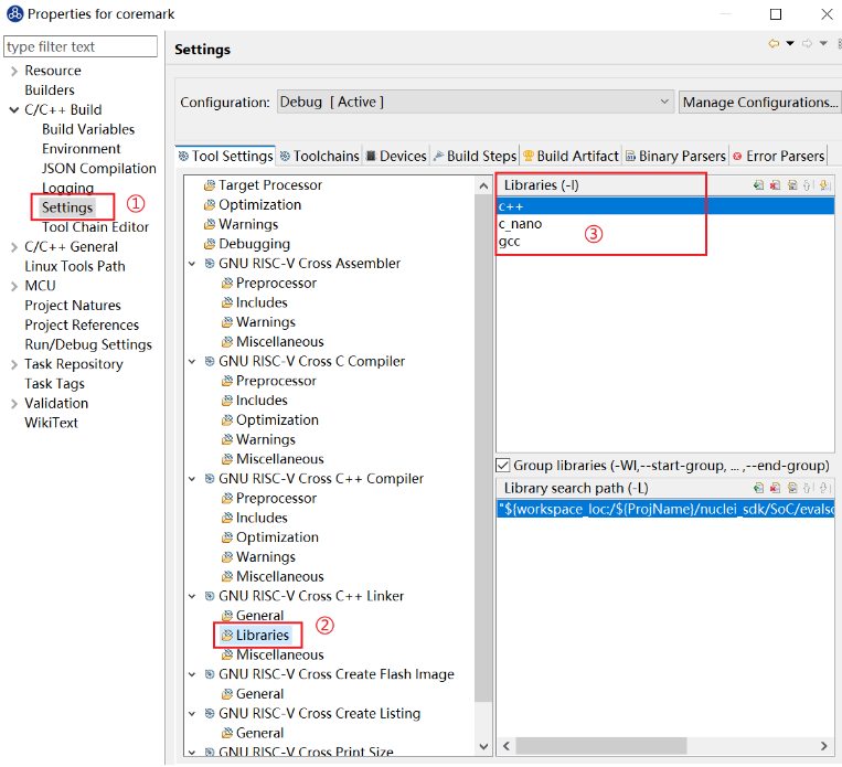
Different toolchains may depend on different libraries, so you also need to check and adjust the linked libraries after switching. The linked libraries can be modified in the project properties under C/C++ Build -> Settings -> Tool Settings -> GNU RISC-V Cross C++ Linker -> Libraries.
For the Clang toolchain, Nuclei Studio still uses the same C standard library, and generally no additional modification of the linked libraries is required. Therefore, when migrating from GCC to Clang, you usually only need to complete the previous two steps, Switching the Toolchain and Adjusting Compile and Link Options, and then try to rebuild the project.
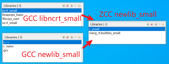
For the ZCC toolchain, the linked library names must also be adjusted. ZCC only supports the newlib_small library, so whether the current GCC project uses newlib_small or libncrt_small, change the linked libraries to c_small and clang_rt.builtins_small.
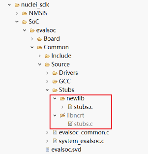
If the current project links libncrt_small, you also need to replace stubs.c with the newlib version; if the project originally uses the newlib library, this step is not needed.
For example, in an EvalSoC project created based on Nuclei SDK, first exclude the libncrt version of stubs.c from the build: select SoC\evalsoc\Common\Source\Stubs\libncrt, right-click and select Resource Configurations -> Exclude from Build..., then copy a newlib version of stubs.c from another project that uses the newlib library into the Stubs directory.
After completing the stubs.c adjustment, the migration from GCC to ZCC is complete, and you can try to rebuild the project.
2.10.16.4. Converting Between newlib_small and libncrt_small
As mentioned earlier, ZCC does not support libncrt_small. Therefore, when switching the toolchain from GCC to ZCC, a project that originally uses libncrt_small must also be switched to newlib_small.
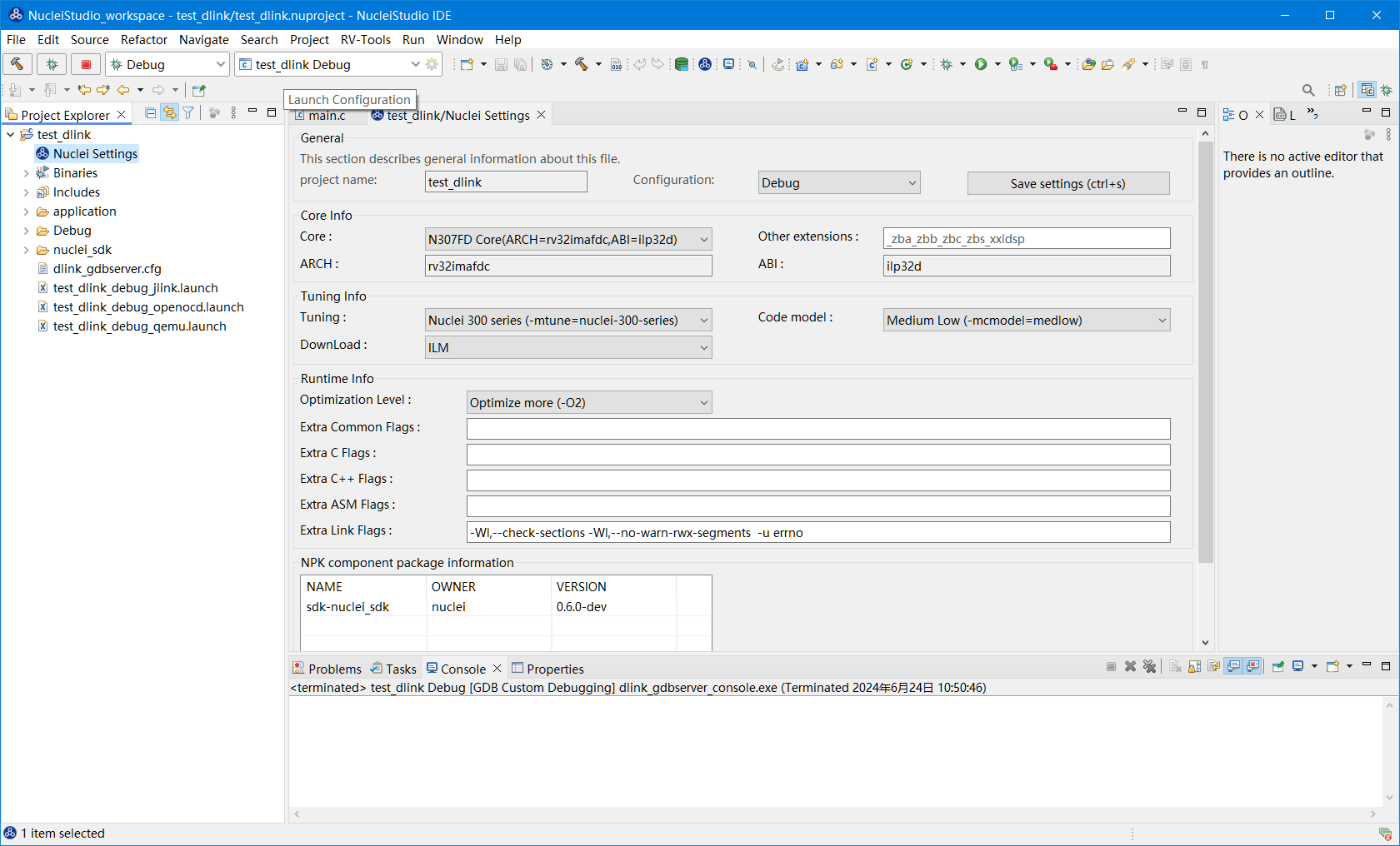
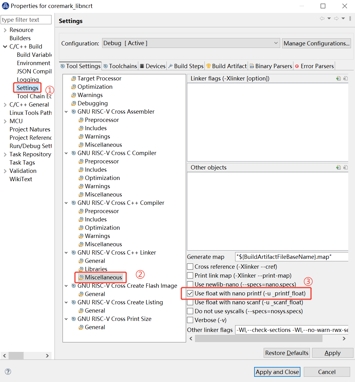
When newlib_small is selected in Nuclei Studio, the actual linked library is c_nano and floating-point printing is supported. -u _printf_float is added to the link options by default. You can check whether this option has been added as shown in the figure below.
The table below summarizes the supported toolchain and C library combinations. When adjusting the toolchain or linked libraries, also check that the Library List, Link Options, and stubs File match.
Toolchain |
Linked Library |
Supported |
Library List |
Link Options |
stubs File |
|---|---|---|---|---|---|
GCC/Clang |
newlib_small |
Supported |
|
-u _printf_float |
newlib/stubs.c |
GCC/Clang |
libncrt_small |
Supported |
|
libncrt/stubs.c |
|
ZCC |
newlib_small |
Supported |
|
newlib/stubs.c |
|
ZCC |
libncrt_small |
Not Supported |
2.10.16.5. Common Issues
2.10.16.5.1. Clang/ZCC Incompatibility with GCC
The Clang/ZCC toolchain is not fully compatible with GCC compile options. If errors are reported during compilation, refer to Adjusting Compile and Link Options for adjustments.
riscv64-unknown-elf-clang: error: unknown argument: '-fno-code-hoisting'
riscv64-unknown-elf-clang: error: unknown argument: '-fno-if-conversion'
riscv64-unknown-elf-clang: error: unknown argument: '-fno-if-conversion2'
riscv64-unknown-elf-clang: error: unknown argument: '-fselective-scheduling'
riscv64-unknown-elf-clang: error: unknown argument: '-fno-tree-loop-distribute-patterns'
riscv64-unknown-elf-clang: error: unknown argument: '-mbranch-cost=1'
The Clang/ZCC toolchain does not support the -Wl,--no-warn-rwx-segments link option. If errors are reported during linking, refer to Adjusting Compile and Link Options for adjustments.
ld.lld: error: unknown argument '--no-warn-rwx-segments'
riscv64-unknown-elf-clang++: error: ld command failed with exit code 1 (use -v to see invocation)
make: *** [makefile:92: coremark.elf] Error 1
2.10.16.5.2. ZCC Link Failures
When switching from GCC to the ZCC toolchain, the following problems may occur if the linked libraries are not adjusted correctly. Refer to Adjusting Linked Libraries for modifications.
If the original project uses newlib_small but the linked libraries are not modified, the following error may occur:
ld.lld: error: unable to find library -lstdc++
z++: error: ld command failed with exit code 1 (use -v to see invocation)
make: *** [makefile:92: coremark.elf] Error 1
If the original project uses libncrt_small but the linked libraries are not modified, the following error may occur:
ld.lld: error: unable to find library -lncrt_small
ld.lld: error: unable to find library -lheapops_basic
ld.lld: error: unable to find library -lfileops_uart
ld.lld: error: unable to find library -lncrt_small
z++: error: ld command failed with exit code 1 (use -v to see invocation)
make: *** [makefile:92: coremark.elf] Error 1
If the original project uses libncrt_small and the linked libraries have been modified, but stubs.c has not been replaced accordingly, the following error may occur:
ld.lld: error: undefined symbol: _read
>>> referenced by ld-temp.o
>>>               coremark.elf.lto.o:(sys_semihost_getc)

ld.lld: error: undefined symbol: _write
>>> referenced by ld-temp.o
>>>               coremark.elf.lto.o:(sys_semihost_putc)
z++: error: ld command failed with exit code 1 (use -v to see invocation)
make: *** [makefile:92: coremark.elf] Error 1